Conditional formatting in MS EXCEL. Conditional Formatting: Microsoft Excel Data Visualization Tool Conditional Formatting by Another Cell Value

Conditional Formatting is a very useful feature in Excel that allows you to format numeric data or text in a table according to given conditions or rules. Thanks to him, by looking at the desired cells, you can immediately evaluate the values, since all the data will be presented in a convenient visual form.

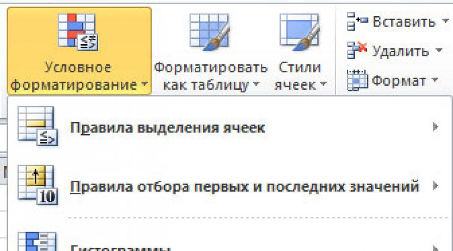
Button "Conditional Formatting" located on the Home tab in the Styles group.

By clicking on it, a menu with types of conditional formatting will open. Let's deal with them in more detail.

Cell selection

In this case, we can compare the numeric data of the selected range of cells with a certain given number, or with another range. You can compare not only numbers, but also text and dates.

Example

Let's compare all the numbers in the selected range and if there are repetitions, paint the blocks with them in a certain color. Click "Conditional Formatting" – "Cell Selection Rules" – "Duplicate Values". Select from the list "recurring" and fill type. Now all repetitions in the column are highlighted in color. As you can see, sixes and eights occur several times in the example.

Now let's compare the data in the first range with the second, and if the number in the first is less, we will highlight the rectangle with a color. Select from the list "Less". Then we make a relative link to the second column: we click on the first number. The dollar in front of F means that we will compare with this column, but in different cells. As a result, all blocks in the first column, where the numbers are written less than in the second, are highlighted in color.

You can also apply formatting to text data. To do this, select from the list "Text contains". For example, let's select all the names that start with "B" - that is, the block itself and the text will be painted in the selected color.

Selecting the first and last values

Using this item, you can select cells that belong to the first or last elements, according to a given number or percentage.

Example

Let's set formatting for those blocks, the value of which is above average in the selected area. Choose from the list "Above average". The corresponding rectangles and the text in them will be highlighted.

Histograms

They show the information in the block in the form of a bar graph. The cell is taken as 100%, which corresponds to the maximum number in the selected range. If the value in the block is negative, the histogram is divided into half, has a different orientation and color.

Example

Let's display the number for each selected block as a histogram. Choose any of the proposed filling methods.

Now let's imagine that the minimum number for building a histogram should be 5. Select the desired range, click on the button "Conditional Formatting" and choose from the list "Rules Management".

The following window will open. In it, you can create a new rule for selected cells, change or delete the one you need from the list. Choose "Change the Rule".

At the bottom of the window, you can change the description for it. We put "Minimum value"- "Number", and in the field "Value" we write "5". If you do not want numbers to be displayed in the cells, check the box "Show column only". You can also change the fill color and type here.

As a result, the minimum number for the selected cells is "5", and the maximum is selected automatically. As you can see in the example, in blocks where the number is less than five: 4, -7, -8, or equal to it, the histogram is simply not displayed.

Color scales

Now let's look at the fourth point. In this case, the cell is filled with a color that depends on the number that is written in it.

If you open a window "Changing a Formatting Rule", as described in the previous paragraph, you can select "Format Style", "Color" of the fill, the maximum and minimum value for the selected range.

For example, in the field "Minimum value" I put "3". The selected area will look like this - blocks with values ​​below 4 will simply not be painted over.

Icon sets

A certain icon will be inserted into the cell, in accordance with its value.

Opening the window "Changing a Formatting Rule", you can select the "Value" and "Type" for the numbers that each icon will correspond to.

How to delete

If you need to remove conditional formatting for a certain range (and not only), click on the button "Remove Rules" and select the desired item from the menu.

How to create a new rule

Button "Create a Rule" will create new necessary conditions for the selected range.

Example

Suppose there is a small plate, which is shown in the figure above. Let's create different rules for it. If the numbers in the range are higher than "0" - paint the blocks in yellow, above "10" - in green, above "18" - in red.

First, you need to select a type - "Format only cells that contain". Now in the field "Change rule description" set the value, select the color of the cell and click "OK". Thus, we create three rules for the selected range.

The table in the example is formatted as follows.

How to manage rules

If you already have conditional formatting in your document and have certain conditions set for it, but you need to change them, then let's look at how to manage them. To do this, select the same range and click on the button "Rules Management".

In this lesson with examples and videos, we will dedicate conditional formatting, one of the most interesting and useful tools in Excel.

What is conditional formatting

So, let's get down to business. Conditional formatting is a way to make it as easy as possible Excel programs. This method of processing information saves a lot of time and facilitates all calculations. You can make the program automatically perform many tasks that you used to do manually, killing whole days for it.

In addition, for your convenience, you can configure Excel job so that he immediately selects the desired or important information in documents. In addition, such formatting will help to display information more clearly, create reports quickly and efficiently without using complex graphical models, such as charts or graphs.

Let's take a look at more concrete examples using conditional formatting. In order to apply it in Excel 10, in the "Home" section on the top panel of the program, you need to find the "Conditional Formatting" button. She is not hiding anywhere, so finding her will not be difficult. In order to activate this formatting, we need to select the zone on the worksheet with which we will work. Keep in mind that before clicking the "Conditional Formatting" button and proceeding with it, you need to select the column, row or several of these elements for which you want to use formatting.

So, the work area is selected, the button is pressed - what's next? A conditional formatting menu will open in front of you, where there will be such items:

1. Rules for selecting first and latest values.
2. Color scales.
3. Optional: create, delete, manage rules.

What to do with it? Let's go in order. This item, in turn, contains such standard functions as

• More;
• Less;
• Equals;
• The text contains;
• Date of;
• Repeating icons.

Working with these formatting models is not difficult at all. By clicking on any of them, you will open a small window where you will need to enter the data you need and select a color to highlight the table cells that suit you.

1. Click "Between" and in the new window that opens, in the appropriate cells, enter the parameters from and to.
2. Then specify the color that you want to highlight the options that suit you (let's say it will be "Light red fill and dark red text"). That is, if you work with a column of prices for Cell phones, then enter the numbers for the minimum and maximum cost, which suits you (let's say it will be 50 and 100).
3. After you have confirmed that it is BETWEEN these values ​​that you want to start searching, the cells in the table will be highlighted accordingly and we will see ALL cells with a price from 50 to 10 dollars colored in light red and with dark red text.

All this is quite easy, when in practice start working with the program.

All formatting methods in the "Cell Selection Rules" menu work in much the same way, so we will not stop here.

Rules for selecting the first and last values

The next item is before us. How it works? If you need to select the first or last few cells according to the entered data, then you are exactly where you need to be. There is nothing more to explain here, so let's move on to an example.

1. By clicking "First 10 elements" we will call up a window where you can control this formatting.
2. Here we indicate the number of cells that we need to select: it was originally named 10, but we only need 5, so we fix this in the corresponding field.
3. Then we choose the formatting color: let it be "Red Border".
4. Then the 5 cells with the largest values ​​will be highlighted with a red frame.

Let's go further. Everything is very simple here. You just need to select the column or line we need and click on the appropriate button. Then we will see how all the cells are more or less filled with color, depending on the values ​​inside them. It's like a real histogram.

• Click "Histogram" and select any model you like in the menu (they differ only in design).
• As a result, our column with the number of phones will change so that the largest digit will have the entire cell filled with color, and all the rest will be filled in as a percentage of the maximum value.

Color scales

They allow us to decorate our cells in ascending or descending order of the values ​​in them. You only need to choose in which color scheme this will happen (for example, the maximum value is green, the minimum is red, and all intermediate values ​​will be colored in the corresponding transitional shades). We won't even give an example here.

Icons are needed in order to indicate the difference between the values ​​in our column or row. Theoretically, it is a bit difficult to explain, so let's immediately move on to examples.

• select "Icon Sets" and in the "Directions" section click on "5 colored arrows". Thus, in each cell of the field in which we work, one of the 5 types of arrow will appear.
• Let's explain how they work: the entire range of values ​​in the cells we have selected is 100%, and each arrow in turn is responsible for the numbers that are included in every 20% in order. Let us have values ​​​​from 0 to 100 in the column for the number of phone purchases. Then the first arrow (green up) will be next to each value from 80 to 100, and the last one (red down) will be next to each value from 0 to 20. Accordingly, all intermediate arrows.

The percentage or the entire range can be configured in the Manage Rules menu, here you can also play around with the settings for the rest of the rules.

Lesson 8

You can change the cell format, remember it, and apply it to another table. First, let's look at the possibilities for formatting a cell. To do this, select several cells, then click on them. right click and call the mode Cell Format.

As you can see, the window contains several tabs. tab Number allows you to specify the format of the data in the cell. It usually rarely changes. As a rule, when entering data into a cell, the program itself determines the format. In fieldNumeric formatsit can be viewed.

Alignment tab allows you to set: where the text will be in the cell. Suppose we typed text into a cell.

As you can see from the figure, the text is adjacent to the left border of the cell. In order to put it in the center, you need to set the parameter in the center in field horizontally .

Interesting mode Orientation , it allows you to print text not horizontally, but in the other direction. Suppose you want to change the direction to the horizontal axis by 45 degrees. To do this, set the arrow in the field Orientation , as shown in fig. below.

As you can see from the figure, the text direction has changed only in the cell to which the mode is applied. In addition, the line size has changed and become larger. There is text in the right cell and it is at the bottom border. To set it elsewhere, select the second cell and use the mode Cell Format, Alignment tab. There in the field vertically set the value - along the top edge.

And the text will move up.

An interesting mode is auto-width, which allows the program to automatically increase the cell size (horizontally and vertically) if the value is out of range. For example, let's increase the font size to 24 in the table created in the previous lessons with the autofit option running.

It can be seen that the vertical size (rows) has changed in the direction of increase. So the lines under the table have smaller size than where there is a table. Note that the type of font in the header is different, as it is increased in size (width) of the cell.

On the Font tab it is possible to set the type of font, its style, size, color, set it as strikethrough, superscript, subscript.

In the example shown above, set the font of the same style in the header (Arial), set it to bold, make it underline, and choose a blue color. To do this, select the header cells and set the parameters as shown below.

In the Sample field you can see what the text will look like.

Now we select the table header again, uncheck the autofit width parameter, and we get the following picture.

As you can see, the text overlaps the text of other cells. Let's use the mode Format on the Home tab.

In the panel that appears, select the modeAutoFit Text Width. We get:

On the Border tab, you can set borders around the cell. Let's say we have several cells, as shown in Fig. below.

Select them and use the tab Border .

We chose the color - orange, the line type - double and pressed the button external.

Now select the table again, and again use the tab Border .

We chose a different color, line type and clicked on the internal button. It was possible not to exit the border setting mode, set the color, line type, press the button external, then change the line type, color and click on the button internal.

Fill tab allows you to set the cell fill. Select the previous cells again and set the color. You can choose a color and then the cells will be filled with a uniform color, but we chose Pattern and to it Pattern color .

Saving cell style . Suppose that we will use the resulting style when creating the following tables. Therefore, select four cells again and click on the button Cell styles on the Home tab.

There are already styles installed in the program, but we need to create our own style. So let's click onCreate cell style.

A window will appear on the screen, in which there are elements for which a style is created, let's call it Try. Check all the checkboxes and click on the button OK . Now the new style will be remembered in the program and when we call the mode Cell styles , then it will appear in the list Custom.

Then, when you need to use the new style, select the cells and use the mode Try . After that new table take on your new style.

Sometimes it is required to allocate numbers depending on certain conditions. So, if the table presents comparative data on categories of the population that abuse certain products, then it is better to highlight persons who are prone to alcoholic beverages in italics, vegetarians who eat food from the garden beds - in underlined font, and those who consume uncontrollably a large number of food is in bold. In addition, the use of a color format may be dictated by certain conditions. For example, if the temperature in an apartment does not rise above 0 in winter, then the number of such apartments should be shown in blue, at a temperature of 0 - 10 degrees - in green, at a range of 10 - 20 degrees - in yellow, and over 30 degrees - in red.

Let's go back to the table we created earlier. Let's select a part of the table with numerical values ​​and use the mode on the tab Home → Conditional Formatting. A mode window will appear on the screen, the view of which is shown in the figure. In this window, select the mode Create rule.

A window will appear in which we set the values ​​for the rules.

Let's set the task to have the background color of the cells depending on their value. Let's choose the upper rule Format all cells based on their values ​​and click on the button OK .

If we change the color to blue, we get the following table.

Select the mode in the style of the format - a three-color scale and click on the button OK .

In these modes, you can change the average value by entering a value using the keyboard, but you can also specify the cell in which this value is located by pressing the - button.

You can set the value bar chart. Then the cells will be filled with the specified color depending on their value.

You can set icons next to the values ​​using the mode - icon sets.

You can perform conditional formatting not on the entire table, but on part of it. There are other modes as well. For example,Conditional Formatting→ Cell selection rules→ Between .

In the window, all values ​​that are between 25 and 72 will be highlighted with a light red fill and a dark red color. These values ​​can be changed by entering them from the keyboard.

In the list of values ​​for which you can change the format, there is a custom format where you can change the font type, style, etc. For example, you can make the style bold.

Note that you can use multiple rules for the same table.

Unformatted spreadsheets can be difficult to read. Formatted text and cells can draw attention to certain parts of the spreadsheet, making them visually more visible and easier to understand.

There are many text and cell formatting tools in Excel. In this lesson, you'll learn how to change the color and style of text and cells, align text, and set a custom format for numbers and dates.

Text formatting

Many text formatting commands can be found in the Font, Alignment, Number groups on the ribbon. Group commands Font allow you to change the style, size, and color of the text. You can also use them to add borders and fill cells with color. Group commands alignment allow you to set the display of text in the cell both vertically and horizontally. Group commands Number allow you to change how numbers and dates are displayed.

To change the font:

1. Select the desired cells.
2. Click the drop-down arrow for the font command on the Home tab. A dropdown menu will appear.
3. Hover your mouse over different fonts. The selected cells will interactively change the font of the text.
4. Choose the font you want.

To change the font size:

1. Select the desired cells.
2. Click the drop-down arrow for the font size command on the Home tab. A dropdown menu will appear.
3. Hover your mouse over different font sizes. The selected cells will interactively change the font size.
4. Choose the font size you want.

You can also use the Increase Size and Decrease Size commands to change the font size.

To use bold, italic, underline commands:

1. Select the desired cells.
2. Click on the command bold (W), italics (K) or underlined (H) in the Font group on the Home tab.

To add borders:

1. Select the desired cells.
2. Click on the command dropdown arrow borders on the home tab. A dropdown menu will appear.
3. Select desired style borders.

You can draw borders and change line styles and colors using the border drawing tools at the bottom of the dropdown menu.

To change the font color:

1. Select the desired cells.
2. Click the drop-down arrow next to the Text Color command on the Home tab. The Text Color menu appears.
3. Hover your mouse over different colors. The sheet will interactively change the text color of the selected cells.
4. Choose the color you want.

The choice of colors is not limited to the drop-down menu. Select More Colors at the bottom of the list to access an expanded Color selection.

To add a fill color:

1. Select the desired cells.
2. Click the drop-down arrow next to the Fill Color command on the Home tab. The Color menu appears.
3. Hover your mouse over different colors. The sheet will interactively change the fill color of the selected cells.
4. Choose the color you want.

To change the horizontal alignment of text:

1. Select the desired cells.
2. Select one of the horizontal alignment options on the Home tab.

• Align text to the left: Aligns text to the left of the cell.
• Align Center: Aligns text to the center of the cell.
• Align text to the right: Aligns text to the right of the cell.

To change the vertical alignment of text:

1. Select the desired cells.
2. Select one of the vertical alignment options on the Home tab.

• Top edge: Aligns text to the top of the cell.
• Align in the middle: Aligns text to the center of the cell between the top and bottom edges.
• Along the bottom edge: Aligns text to the bottom of the cell.

By default, numbers align to the right and bottom of the cell, while words and letters align to the left and bottom.

Formatting numbers and dates

One of the most useful Excel functions is the ability to format numbers and dates different ways. For example, you may want to display numbers with a decimal separator, a currency or percentage symbol, and so on.

To set the format for numbers and dates:

Numeric Formats

1. General is the default format of any cell. When you enter a number in a cell, Excel will suggest the number format that it thinks best. For example, if you enter "1-5", the cell will display a number in the Short Date format, "1/5/2010".
2. Numerical formats numbers to decimal places. For example, if you enter "4" in a cell, the number "4.00" will be displayed in the cell.
3. Monetary formats numbers in display form currency symbol. For example, if you enter "4" into a cell, the number will be displayed as "" in the cell.
4. Financial formats numbers similar to the Currency format, but additionally aligns currency symbols and decimal places in columns. This format will make long financial lists easier to read.
5. Short date format formats numbers as M/D/YYYY. For example, the entry August 8, 2010 would be represented as "8/8/2010".
6. Long date format formats numbers as Day of Week, Month DD, YYYY. For example, "Monday, August 01, 2010".
7. Time formats numbers as HH/MM/SS and signed AM or PM. For example, "10:25:00 AM".
8. Percentage formats numbers to decimal places and a percent sign. For example, if you enter "0.75" into a cell, it will display "75.00%".
9. Fractional formats numbers as fractions with a slash. For example, if you enter "1/4" into a cell, the cell will display "1/4". If you enter "1/4" into a cell with the General format, the cell will display "4-Jan".
10. Exponential formats numbers in scientific notation. For example, if you enter "140000" into a cell, the cell will display "1.40E+05". Note that by default, Excel will use exponential format for a cell if it contains a very large integer. If you don't want this format, then use Number Format.
11. Text formats numbers as text, that is, everything in the cell will be displayed exactly as you entered it. Excel uses this format by default for cells that contain both numbers and text.
12. You can easily customize any format using the Others item. number formats. For example, you can change the US dollar sign to another currency symbol, change the display of commas in numbers, change the number of decimal places to display, and so on.

Conditional formatting in Excel is a great tool for quick visual analysis of data. In this way, it is much more convenient and easier to evaluate information. Moreover, all this takes place in automatic mode. The user does not need to think and compare values ​​on his own. The editor will do everything himself. In no formula you can do what this tool can do.

In order to use this feature, you need to go to the "Home" tab and click on the "Conditional Formatting" button.

Back to main sections this menu relate:

• cell selection rules;

• rules for selecting the first and last values;

• histograms;

• color scales;

• icon sets;

Let's take a closer look at these points. To do this, we will create some kind of table in which it will be possible to compare numerical values.

This section also has a lot of different formatting options. Let's analyze each of them.

More

1. To get started, select a line. In this case, it will be the victims in the first mine.

1. Then go to the "Home" tab and click on the "Conditional Formatting" button. In the menu that appears, click on the item "Cell Selection Rules". Then select the "More" option.

1. After that, a window will appear in which you need to specify a value for comparing the selected elements. You can enter anything or click on any cell. Click on the average. This indicator is quite suitable for comparison.

1. Immediately after that, the link to the cell will be substituted automatically (and it will be highlighted dotted line). To paste, click on the "OK" button.

1. As a result of this, we will see that the cells in which the value is greater than 27 are highlighted in a different color.

If you don't like the cell fill color, you can always change it. To do this, you need to select any other coloring option at the stage of specifying a number for comparison.

If you do not like any of the proposed options, you can click on the "Custom Format ..." item.

Immediately after that, a window will appear in which you can specify the cell format you need.

1. Select a line. Click on the Conditional Formatting icon located on the Home tab. Select "Cell Selection Rules" and then "Less Than".

1. You will again be prompted to specify a cell to compare. To do this, left-click on the desired cell.

1. As a result of this, the desired address will be substituted. To save the settings, click on the "OK" button.

1. As a result of this, we see that all cells whose value is less than 24 are highlighted in a different color.

1. Select some line without formatting rules. We go to the same menu section, but this time we select the “Between” item.

1. Then the Excel editor itself will offer some intermediate values. You can leave everything unchanged.

1. Or substitute something of your own, which is more convenient for you. For example, more than 14, but less than 17. To save, click on the "OK" button.

1. As a result of this, everything that is between these numbers is highlighted in a different color.

1. Select another cell that is free from formatting. We make the same path on the toolbar and select the "Equals" item.

1. We will be asked to provide a link to a cell for comparison or a ready-made numeric value. Let's enter, for example, the number 18. Since it occurs in the selected line. To save, click on the "OK" button.

1. Due to this, the cell that corresponds to the specified value has become highlighted in a different color.

1. To check, you can try to change something. For example, let's take a neighboring cell. Let's fix 19 by 18 there. After pressing the Enter key, you will see the following.

We see that the background of the cells changes completely automatically.

Text contains

The steps above are only suitable for numeric values. To work with text information you need to choose another tool.

1. First of all, select a line with several numbers. Then, using the familiar menu, select "Text contains ...".

1. As a result of this, a window will appear in which you need to specify some piece of text. It can be a letter or a number. Let's use the number "2" as an example. Click the OK button to save the formatting.

1. As a result of this, cells with the numbers 20 and 23 stand out, since both of them have the number 2.

Similar manipulations can be done with temporary values.

1. First, let's add a line in which we write several dates. It is desirable that they go in a row. This will make it easier to compare.

1. After that, select this entire line. Then go to the "Conditional Formatting" menu and select "Date".

1. Immediately after that, a window will appear in which you can select several options:
   • yesterday;
   • Today;
   • Tomorrow;
   • for the last 7 days;
   • last week;
   • this week;
   • next week;
   • last month;
   • this month;
   • next month.

1. As an example, let's choose the option "Tomorrow". Click the "OK" button to save.

1. As a result, the field containing tomorrow's date will be highlighted in a different color.

1. The current date at the time of writing is February 25, 2018.

To demonstrate this conditional formatting, it is desirable to use a table without other comparison rules. Next, you will need to perform the following steps.

1. Highlight the main values ​​in the table that need to be analyzed somehow.

1. Click on the "Conditional Formatting" icon and in the "Cell Selection Rules" select "Duplicate Values".

1. Immediately after that, a window will appear in which you can select two values:
   • recurring;

• unique.

In each case will be available preview so you can figure out exactly what you need. To save, click on the "OK" button.

In addition to the usual selection of specific numbers, there is the possibility of marking a certain amount elements in percentage or quantitative ratio. To do this, do the following.

1. Highlight the contents of the table. Then you need to click on the "Conditional Formatting" button, which is located on the "Home" tab. After that, select the "Rules for selecting the first and last values" item. As a result, you will be offered several selection options.

Let's consider each of them.

By selecting this item, you will see a window in which you will be asked to specify the number of first cells. Click "OK" to save.

The countdown is from a larger value to a smaller one.

This means that if you need to select the first 10 cells in which the smallest numbers are located, then you need to select the “Last 10 elements” item.

While entering the number of cells, a preview will be available to you. If you specify the number 1, then only 1 maximum value will remain.

Please note that if there are two cells with the same maximum number, both will be selected!

In this case, everything works almost according to the same principle, only this time it is not a specific fixed number of cells that are highlighted, but only a certain percentage of them.

If you specify the number 10 (it is used by default), then you will see the following.

If this rule formatting you like, you need to click on the "OK" button. Otherwise, click on Cancel.

Last 10 items

As mentioned above, in this case, those cells that contain the minimum data are selected. The input principle is the same - specify the desired amount and click on the "OK" button.

If you specify only 1 cell, but there will be several minimum digits, then all will be selected (in our case, two).

The same principle, only this time a certain percentage of information is highlighted, and not an absolute amount.

This tool is very handy when you need to sort information in relation to itself. That is, the Excel editor itself will calculate the average number among the selected information and mark everything that is above this value. Everything happens automatically.

A similar principle of action in this case. Only this time, cells are marked in which information is stored less than the average value.

In the methods of data comparison described above, the method of continuous filling of elements was used. Sometimes this is not very convenient.

For more advanced information analysis, another tool is used - histograms. In this case, the filling can be of two types:

• gradient;
• solid.

Let's consider each of the proposed options.

gradient fill

1. The first step is to select the desired rows and columns. Then click on the Conditional Formatting icon. After that, go to the "Histograms" section and select any of the proposed fills.

The default values ​​are:

• green;
• red;
• orange;
• blue;
• purple.

Hovering over each option will give you a preview.

This type of marking does not differ much from the one described above and is located in the same section.

The colors used are the same.

If you do not like any of the proposed items, you can specify your formatting option.

Here you can configure:

• style;

• minimum and maximum value;

• appearance column.

A sample of what you have configured can be seen in the lower right corner.

If you want something more contrast, you need to do the following.

1. Highlight the table (basic information for data analysis). Click on the "Conditional Formatting" icon, which is located on the "Home" tab on the toolbar. In the menu that appears, select "Color Scales". As a result of this, a large list of 12 design options will appear.

1. When you hover over each template, you will see a similar explanation.

When you hover over each of the icons, a preview will be available to you. So you can choose the color scheme that you like the most.

If you didn’t like anything suggested by the Excel editor, you can always create something of your own. To do this, in the same section of the menu, click on the item "Other rules".

Right after that, you will see the following window. Here you can specify the start and end color. To save, just click on the "OK" button.

If you don't like the color formatting, you can use the graphical method. To do this, you must do the following.

1. Select the main cells of the table.
2. Click on "Conditional Formatting" in the toolbar.
3. From the menu that appears, select the Icon Sets category.
4. Immediately after that, you will see a large list of different templates.

It should be noted that the editor itself automatically divides the data into several groups: minimum, average and maximum.

The options are (each time you hover over any icon you will see a preview without saving the formatting rule):

• directions (an up arrow will appear near large numbers; to the right for medium numbers; the downward direction corresponds to the minimum numbers);

• shapes (color depends on the number in the cell - grey colour for the largest values);

• indicators (tick - high, Exclamation point- average, and a cross - a minimum);

• estimates (the degree of filling of the element depends on the number in the cells);

If you don't like any of the icons, you can create your own cell filling rule.

In this case, you can specify the following parameters yourself:

• icon style;

• your version of the icon;

• boundary values ​​for icons;

Click the "OK" button to save.

If your experiment failed and the manipulations you did only spoiled the appearance of the table, then all this can be canceled in a fairly simple way.

1. First you need to select those elements whose conditional formatting you want to disable.

1. Then click on the "Home" tab on the "Conditional Formatting" icon.
2. Then select "Delete Rules".
3. Next, click on "Remove rules from selected cells".

1. If you want to delete everything, then select the second item - "Delete rules from the entire sheet."

1. The result will be the following. Everything will return to its original form.

The set of formatting methods can be changed at will. This is done in the following way.

1. Click on the "Conditional Formatting" button.
2. Select Manage Rules.

1. There will be nothing in the rule manager that appears (if you did not select anything before calling this menu), since the “Current Fragment” item is selected by default.

1. Select "This sheet".

1. As a result, you will see all the rules that are currently used in the document.

Removal

In order to delete something, just select something from the list and click on the "Delete rule" button.

You need to be very careful when performing such actions, since you will not be additionally asked if you are sure of your choice.

Change

Editing the rules is pretty easy. This is done in the following way.

1. Select any line.
2. Click on the "Edit Rule" button.

1. As a result, you will see the following window. The default type is "Format only cells that contain".

1. Here you can specify what exactly they contain:
   • text;
   • dates
   • empty;
   • non-empty;
   • errors;
   • no mistakes.