How to make number format in excel. Automatic cell format change after data entry

Changing the cell format in Excel allows you to organize the data on a sheet into a logical and consistent chain for professional work. On the other hand, incorrect formatting can lead to serious errors.

The contents of a cell is one thing, but the way the contents of the cells are displayed on the monitor or printed is another. Before you change the data format in an Excel cell, you should remember a simple rule: "Everything that the cell contains can be presented in different ways, and the presentation of the data display depends on the formatting." This is easy to understand if shown with an example. See how you can use formatting to display the number 2 in different ways:

Most Excel users use exclusively standard tools formatting:

• buttons on the Home panel;
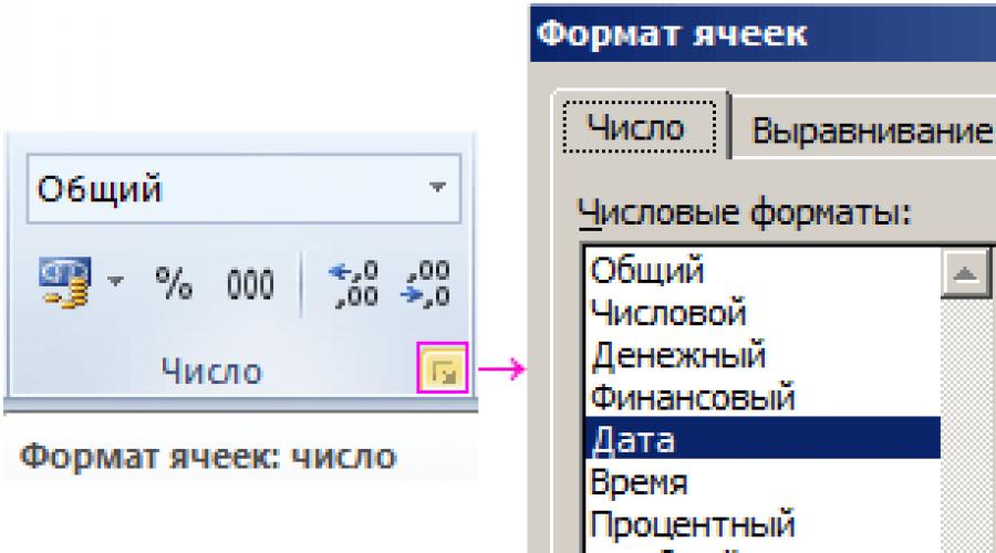
• ready-made cell format templates available in the dialog box are opened using the CTRL + 1 hot key combination.

Data formats entered into spreadsheet cells

Fill in the cell range A2:A7 with the number 2 and format all cells as shown in the figure above.

The solution of the problem:

What options does the Format Cells dialog box provide? The functions of all the formatting tools that the Home tab contains can be found in this dialog box (CTRL+1) and even more.

In cell A5, we used the financial format, but there is also a monetary format, they are very often confused. The two formats differ in the way they are displayed:

• the financial format, when displaying numbers less than 0, puts a minus on the left side of the cell, and the money format puts a minus in front of the number;
• the default currency format displays negative values ​​in red font (for example, enter the value -2p in the cell and the currency format will be assigned automatically);
• in financial format, 1 space is added after currency reduction when displaying values.

If you press the hotkey combination: CTRL + SHIFT + 4, then the cell will be assigned the monetary format.

As for the date in cell A6, it's worth mentioning the Excel rules here. The date format is considered as a sequence of days from January 1, 1900. That is, if the cell contains a value - the number 2, then this number in the date format should be displayed as 01/02/1900 and so on.

Time for Excel is the value of numbers after the decimal point. Since we have an integer in cell A7, the time is displayed there accordingly.

Date format with time in Excel

Let's format the data table so that the values ​​in the rows are displayed according to the column names:

In the first column, the formats already correspond to its name, so go to the second and select the range B3:B7. Then press CTRL + 1 and on the "Number" tab, specify the time, and in the "Type:" section, select the display method as shown in the figure:

We do the same with the ranges C3:C7 and D3:D7, choosing the appropriate formats and display types.

If the cell contains a value greater than 0 but less than 1, then the date format in the third column will be displayed as: January 0, 1900. While in the fourth column the date is already displayed differently due to a different type (1904 date systems, see below for details). And if the number

Notice how the time is displayed in cells that contain fractional numbers.

Since dates and times in Excel are numbers, it is easy to perform mathematical operations with them, but we will consider this in the next lessons.

Two Excel date display systems

There are two systems for displaying dates in Excel:

1. The date January 1, 1900 corresponds to the number 1.
2. The date January 1, 1904 corresponds to the number 0, and 1 is already 01/02/1904, respectively.

Note. In order for all dates to be displayed by default according to the 1904 system, you can make the appropriate settings in the parameters: “File” - “Options” - “Advanced” - “When recalculating this book:” - “Use the 1904 date system”.

We clearly give an example of the difference in the display of dates in these two systems in the figure:

The Excel help lists the minimum and maximum numbers for dates in both systems.

The settings for changing the date system apply not only to a specific sheet, but to the entire program. Therefore, if there is no urgent need to change them, then it is better to use the default system - 1900. This will avoid serious errors when performing mathematical operations with dates and times.

Excel has many built-in number formats, but if none of them satisfies the user, then you can create your own number format. For example, the number -5.25 can be displayed as a fraction -5 1/4 or as (-)5.25 or 5.25- or, in general, in an arbitrary format, for example, ++(5)rub.###25kop. The formats of monetary amounts, percentages and exponential representation are also considered.

You can use many formats to display a number. According to Russian regional standards ( Start Button/ Control Panel/ Regional and Language Options) the number is usually displayed in the following format: 123 456 789.00 (digits are separated by spaces, the fractional part is separated by a comma). In EXCEL, you can come up with the format for displaying a number in a cell yourself. There is an appropriate mechanism for this - a custom format. Each cell can be set to a specific number format. For example, the number 123,456,789.00 has the format: # ##0,00;-# ##0,00;0

The custom number format does not affect calculations, only the display of the number in the cell changes. Custom format can be entered through the dialog box Cell Format, tab Number, (all formats) by pressing CTRL+1. Enter the format in the field Type, after deleting everything from it.

Let's start with the standard number format mentioned above # ##0,00;-# ##0,00;0
In the future, we will learn how to change it.

Semicolons separate parts of the format: format for positive values; for negative values; for zero. Special characters are used to describe the format.

• The pound sign (#) means any number.
• Space character in construction # ##0 defines the digit (a space indicates that there are 3 digits in the digit). In principle, one could write # ###, but zero is needed to display 0 when the integer part is zero and there is only a fractional part. Without a zero (i.e. # ###) the number 0.33 will be displayed as .33.
• The next 3 characters, 00 (comma and 00) determine how the fractional part will be displayed. Entering 3.333 will display 3.33; when entering 3.3 - 3.30. Naturally, this will not affect the calculations.

The second part of the format is for displaying negative numbers. Those. You can set different formats to display positive and negative numbers. For example, with the format # ##0.00;-###0;0, the number 123456.3 will be displayed as 123456.30, and the number -123456.3 as -123456. If you remove the minus format, then negative numbers will be displayed WITHOUT MINUS.

There is also a 4th part - it determines the output of the text. Those. if in a cell with a format # ##0.00;-# ##0.00;0;"You have entered text" enter a text value, it will be displayed You have entered text.

For example, the format 0;\0;\0;\0 allows you to replace all negative, equal to zero and text values to 0. All positive numbers will be displayed as integers (with normal rounding).

It is not necessary to include all parts of the format (section) in the generated number format. If only two sections are specified, the first section is used for positive numbers and zeros, and the second section is used for negative numbers. If only one section is given, all numbers will have this format. If you want to skip a section of code and use the section that follows it, you must leave a semicolon in your code that ends the section you are skipping.

Let's consider custom formats with specific examples.

Having such an advanced custom format is a legacy from previous versions EXCEL that didn't have . Formats that change the font color and background of a cell depending on the magnitude of the value are better implemented conditional formatting.

More complex examples custom formatting is provided in the example file.

Can't recommend using custom format too often. Firstly, 90% of the built-in formats are enough, they are clear to everyone and easy to use. Secondly, as a rule, a custom format can significantly change the display of a value in a cell from the value itself (otherwise, why else would a custom format be needed?) For example, the number 222 can be displayed as "ABCD333-222". You can forget and confuse that the cell contains not text, but not just a number. And this is already possible reason errors. Weigh the pros and cons before using a complex custom format.

The cell format includes parameters that determine: » the type of representation of the numeric value of the cell; » cell content alignment and orientation; » type of font; « cell framing; filling (background) of the cell. In addition, you can set the protection settings for the data written to the cell. Cells are usually formatted by changing individual

parameters. Before you can change the format of a cell, you must place a table cursor on it. If you want to set the format for several cells at the same time, you must first select these cells.

Standard Formats Excel has six standard cell formats (sets of options) that can be used in all documents. new table all cells have the same standard format The default. This format is called Normal. It has the following options:

The depicted value repeats the true value;

Horizontal alignment depends on the type of data;

Vertical alignment is performed on the bottom edge;

Text without word wrap;

The displayed value orientation is horizontal;

Content is displayed in a standard font without highlights or effects;

There is no border around the cells;

There is no filling.

The rest of the standard formats differ from the Normal format only by displaying numbers in cells:

Financial (or Separated) - the number is rounded to two decimal places, for example, the number 43.569 is represented as 43.57;

Financial(0) - the number is rounded to the nearest integer, for example, the number 43.569 is represented as 44;

Monetary - the number is rounded to two digits after the decimal separator and a currency sign is added, for example, the number 43.569 on a "Russian" computer is represented as 43.57 rubles;

Monetary (0) - the number is rounded off as a whole and a currency sign is added, for example, the number 43.569 is represented as 44 rubles;

Percentage - if a number from 0 to 1 is entered into the cell after setting the format, then it is multiplied by 100, then the number (regardless of the value) is rounded to an integer and a% sign is added to it, as a result of this, for example, the numbers 0.43569 and 43.569 will be represented equally by 44%. If in the Options dialog box on the Edit tab, turn off the Automatic input, percent switch, then all numbers will be multiplied by 100, and not just from 0 to 1. As a result of this, for example, the numbers 0.43569 and 43.569 will be represented as 44% and 4357%. The same will happen if this switch is enabled, but the numbers were entered into the cells before they were assigned the Percentage format.

When using financial and monetary formats, the separator between the digits of units, thousands, millions, etc. is set in the Windows settings: the Numbers tab in the Language and Standards program in the Control Panel. This is usually a space. At Windows setup the sign of the currency unit is also set: the Currency tab in the Language and Standards program on the Control Panel. For the ruble, this is usually r. The thousands separator used can be changed without changing the general setting Windows.

To do this, in the Options dialog box, on the International tab, in the Numbers group, turn off the Use system separators switch and enter a different separator in the Digit separator field. Sometimes a comma or an apostrophe is used as such a separator. To apply standard formats, the corresponding tools of the Formatting panel and keyboard shortcuts, as well as the Style dialog box, can be used. Representation of a numeric value As already noted, the values ​​after they are entered into the cells have the form set by default.

However, it is possible to change the appearance of the cells as you wish. You can use the Formatting toolbar and keyboard shortcuts to change individual settings. However, the Format Cells dialog box provides the most complete cell formatting options. To call the Format Cells window, do one of the following:

Run command Cells...(Format);

Run Format Cells... context menu cells (selected cells);

Press the combination Ctrl + 1.

On the Number tab of the Cell Format window, the Number formats list contains the names of the groups of representations of numeric values ​​available in Excel. By default, the list is set to General, which displays numeric values ​​as entered by the user. After selecting a different value, the tab displays additional options, with the help of which the parameters of the appearance of numerical values ​​are set.

For example, when you select Numeric, the following appears:

Field Number of decimal places - setting the number of characters after the decimal separator;

Thousands separator switch - enable the digits separator (space) between groups of digits of units, thousands, millions, etc.;

List Negative numbers - selection of the type of representation of negative numbers. When choosing a format, it is convenient to use the Sample field, which changes in accordance with changes in the tab options. If the value (all formats) is selected in the Number formats list, then the Type list appears, which includes all available number formats, which, however, are written as codes ( symbols). Having dealt with these codes, the user in the Type field can independently set the formats.

So, for example, the following notation is used in format codes:

An optional digit, i.e. if there is no digit in place of the # sign in the number, then nothing is displayed in this place;

Mandatory digit, i.e. if there is no digit in place of the 0 sign, then zero is displayed in this place (usually, the output of zeros after the decimal separator is set in this way, for example, the format 0.000 sets the mandatory display of three characters after the separator);

Mandatory place, i.e. if in place of the sign? there is no digit in the number, then a space is displayed in this place (usually this ensures the alignment of numbers in one column, for example, the format ?????0.00 sets the alignment to the decimal separator of all numbers that have up to six digits before the separator); h, hh, m, mm, s, ee, D, DD hours, minutes, seconds and days of the month (when using a single-letter designation, numbers less than 10 are displayed without a leading zero, i.e., for example, the time 6 hours 5 minutes in the format h:m will look like 6:7, and in the format hh:mm - 06:07); M, MM, MMM, MMMM month (for example, February in different formats will look like 2.02, fairy, February); IT, YYYY year (recorded using 2 or 4 digits, respectively).

Separators in date and time formats are determined by the settings specified in the Windows settings:

the Date and Time tabs in the Language and Standards program in the Control Panel. More detailed information about the notation used in the codes can be found in help system Excel. The user-created format can then be deleted by clicking the Delete button. When changing the format of numerical values, their true values ​​(entered or calculated by formulas) do not change, i.e., for example, no matter how many decimal places are displayed, all available characters will be used in formula calculations.

In other words, setting a new format only changes appearance numeric value without changing its value. At the same time, it is possible to set such a mode in which the accuracy of the true values ​​will always be equal to the accuracy of the representation of numbers on the screen. To do this, in the Options dialog box, on the Calculations tab, in the Book Options group, turn on the screen accuracy switch. This setting will apply to all tables in the book.

To set the format of numerical values, the Formatting panel can be used, on which the following tools are located:

Monetary Format Set the standard format to Monetary;

Percent Format Set the default format to Percentage;

Delimited Format Sets the standard format Financial,

Increase bit depth increase by one the number of characters after the decimal separator;

Decrease bit depth..;

decrease by one the number of characters after the decimal separator. Keyboard shortcuts for setting numeric value formats:

Ctrl+Shift+" .... set the format to Normal;

CtrI+Shift+1 ... set the number format to 0.00 with a separator of groups of digits;

Ctrl+Shift+2.... set time format to hmm;

Ctrl+Shift+Z.... set the date format to DD. MMM.YY;

Ctrl+Shift+4.... set the format to Monetary;

Ctrl+Shift+5.... set format Percentage;

CtrI+Shift+6.... setting the format to 0.00E+00 (exponential view). If a numeric value is entered in a cell, but you want it to be interpreted by the program as a text value, then for such a conversion in the Cell Shape dialog box on the Number tab, in the Numeric formats list, select the Text value.

When filling out sheets excel data, no one can immediately fill everything beautifully and correctly on the first try.

In the process of working with the program, something constantly needs to be changed, edited, deleted, copied or moved. If erroneous values ​​are entered into the cell, naturally we want to correct or delete them. But even such a simple task can sometimes create difficulties.

How to set cell format in Excel?

The content of each Excel cell consists of three elements:

1. Meaning: text, numbers, dates and times, boolean content, functions and formulas.
2. Formats: border type and color, fill type and color, how values ​​are displayed.
3. Notes.

All three of these elements are completely independent of each other. You can set the cell format and do not write anything to it. Or add a note to an empty and unformatted cell.

How to change cell format in Excel 2010?

To change the cell format, call the corresponding dialog box by pressing CTRL + 1 (or CTRL + SHIFT + F) or from the context menu after clicking the right mouse button: the “Format Cells” option.

There are 6 tabs available in this dialog box:

If you did not achieve the desired result on the first try, call this dialog box again to correct the cell format in Excel.

What formatting is applicable to cells in Excel?

Each cell always has some kind of format. If there were no changes, then this is the "General" format. It is also standard Excel format, in which:

• numbers are right-aligned;
• text aligned to the left side;
• Colibri font with a height of 11 points;
• the cell has no borders and no background fill.

Deleting a format is a change to the standard "General" format (without borders and fills).

It is worth noting that the format of cells, unlike their values, cannot be deleted with the DELETE key.

To remove the cell format, select them and use the "Clear Formats" tool, which is located on the "Home" tab in the "Editing" section.

If you want to clear not only the format, but also the values, then select the “Clear All” option from the drop-down list of the tool (eraser).

As you can see, the eraser tool is functionally flexible and allows us to make a choice of what to delete in the cells:

• content (same as the DELETE key);
• formats;
• notes;
• hyperlinks.

The Clear All option combines all of these features.

Deleting notes

Notes, as well as formats, are not deleted from the cell with the DELETE key. Notes can be deleted in two ways:

1. Eraser Tool: Clear Notes option.
2. Right-click on the cell with the note, and select the "Delete note" option from the context menu that appears.

Note. The second way is more convenient. When deleting several notes at the same time, you must first select all their cells.

Need to change the default format to something else

Cell Data Format

Default Cell Format ("General")

By default, after a document is created, all cells are in the General format. This format has a number of tricks:

• numbers are right-aligned and text is left-aligned;
• if, by changing the width of a column, to make it less than a certain one, then the number in the cells is replaced by the characters "#". It's not a mistake. This means making the column wider;
• if the number is very large ("6000000000000") or very small ("0.00000000000001"), it is automatically converted to exponential (scientific) format ("6E+12" and "1E-14" respectively);
• decimal fractions are rounded when the column width is changed. For example, if you write "3.1415", then change the width so that "5" no longer fits, the cell will display "3.142".

Often you need to add a currency symbol, a percent sign to a number in a cell, set the number of decimal places, present a date in a certain format, etc.

Do not add symbols of monetary units manually! After that, it may turn out that when you try to use the value from this cell in the formula, Excel will give an error! There is a way to tell Excel that the cells are in a certain format, and it will automatically add currency symbols (and not only) for us.

There are 3 ways to change the format of data representation in cells:

1. automatically after entering certain data into a cell, Excel itself will change the cell format;
2. using the buttons on the Formatting toolbar.
3. using the "Format Cells" window;

After entering certain sequences characters, Excel automatically formats the cell. After that, everything subsequently entered into this cell excel numbers tries to convert to this format.

• date. If you write "1.2.3" or "1/2/3" in a cell, Excel will replace it with "02/01/2003" (the first day of the second month of the third year). If you write "1.2" or "1/2", then Excel will replace it with "01.Feb". In this case, the cell format will be automatically converted to "Date";
• Percentage. If you write "1%" in a cell, the cell format will automatically change to "Percent";
• Time. If you write "13:46:44" or "13:46" in a cell, the cell format will automatically change to "Time";

Attention!!! on different computers the default formats for representing numbers, currencies, dates and times may differ! You can configure them along the path "Control Panel" -> "Regional and Language Options" -> "Regional Settings" tab.

Changing the format of cells using the buttons on the Formatting toolbar

There are 5 buttons on the "Formatting" toolbar with which you can quickly change the format of selected cells.

Description of buttons (from left to right):

• Money format. The default currency will be used (see above);
• Percent Format. If the cell already contains a number, Excel will multiply it by 100 and add a "%" sign. That's right, because 1 watermelon is "100%", and "0.7" watermelon is "70%";
• Delimited Format (Number Format). In this format, groups of digits (hundreds, hundreds of thousands, etc.) will be separated by a space and 2 decimal places will be added;
• Increase bit depth. Adds one decimal place;
• Decrease bit depth. Removes one decimal place.

Changing the Format Using the Format Cells Window