How to plot a function in Microsoft Excel. How to plot graphs and charts in Excel Graphing a function

Excel is great at building any graphs and charts.

How to build a graph in Excel 2007

For example, let's build a graph of the function y=x(√x-3) on the segment .
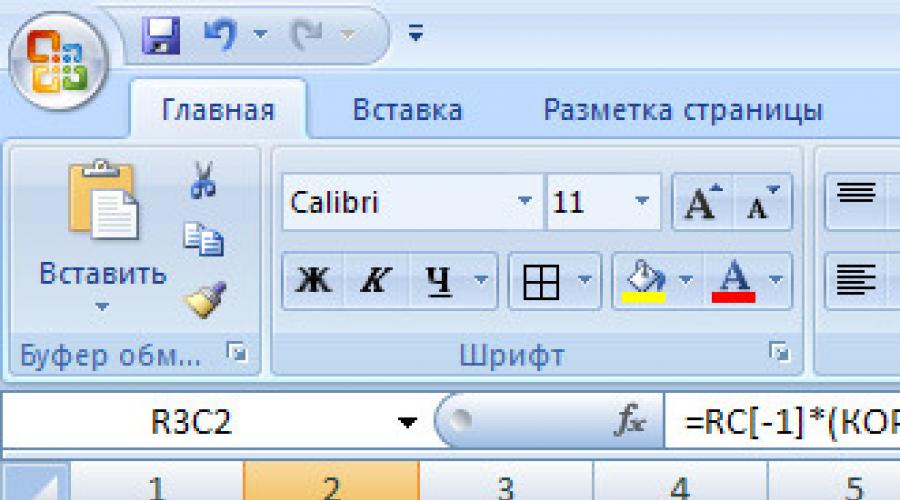
We create a table with two columns. In the first column we will have the values ​​of the argument, and in the second we will have the calculated values ​​of the function. The argument column is filled with values ​​on a given interval with a step of 0.5. And in the cell R3C2 of the function column, we put the formula for its calculation.

After pressing Enter in cell R3C2, the value of the function will be calculated. Let's make this cell active again and move the cursor to the lower right corner so that it changes its appearance to a black cross. Click the mouse and move the cursor down to the last line of the plate. This will copy the formula to all cells.

We got a table filled with function values. Select the cells of the column with its values ​​and go to the "Insert" tab of the top panel.


We press the "Graph" button, select any type that suits us, and we get the graph.


Everything is fine with the Y-axis, but the X-axis contains not the values ​​of the argument, but the numbers of the points. To fix this, right-click on it - "Select Data".


Click on the button that changes the labels of the horizontal axis and select the range with the argument values.


Now our schedule has acquired the proper form.

How to do it in Excel 2003

The beginning is the same, but we can call the diagram wizard by selecting the "Charts" item in the "Insert" menu.


This wizard sets the type and appearance future graph, as well as the labels of the axes.
Conquer Excel and see you soon!

We have already said many times that Excel is not just a program whose tables can be filled with data and values. Excel is multi tool that you just need to know how to use. On the pages of the site, we give answers to many questions, talk about functions and features, and now, we decided to tell you how build a graph in excel 2007 and 2010. Just recently there was an article, and now the time has come to Excel. It does not matter what kind of graph it will be - with two or more variables, you need to study or write a report on work. IN Microsoft Excel you can build any according to your needs, while giving it a great look.

To build a graph in Excel, we decided to take an example when an author sells several of his books and writes down how much profit they brought him in a given month. You, of course, make charts from your data.

We build graphs by points in Excel 2007. Practice

And so, let's go directly to the practical part.

We have already entered all the data in the tables and we are ready to plot.

1. Select any cell outside the table and go to top menu to the Insert tab.

2. Click on the Charts picture in the same menu and select the view in which you would like to get the plotted chart.

3. Then click on the Select data button - all in the same top menu.

4. Then, we completely select all our cells along with symbols and data (as in the figure below).

As we can see, when choosing a data source, we have swapped categories and rows, so we should click on the “Row \ Column” button.

That's all, we have built a graph in Excel 2007, where each value has its own point.

If some values ​​and data need to be corrected, feel free to change them in the corresponding cells. Naturally, the schedule will immediately change.

“Tuning” the constructed graph

If you don't like the resulting chart, it's okay from a visual standpoint. You can choose any of the offered Microsoft Excel, as well as change the colors of points and graphs.

To do this, click on the chart or on any of its elements and click “Change chart type…”

Plotting a function in Excel is not a difficult topic and Excel can handle it without problems. The main thing is to set the parameters correctly and choose the appropriate diagram. IN this example Let's build a scatter plot in Excel.

Considering that the function is the dependence of one parameter on another, we set the values ​​for the x-axis with a step of 0.5. We will build a graph on the segment [-3; 3]. We call the column "x", write the first value "-3", the second - "-2.5". Select them and drag down the black cross in the lower right corner of the cell.

We will plot a function of the form y=x^3+2x^2+2. In cell B1 we write "y", for convenience, you can enter the entire formula. Select cell B2, put "=" and write the formula in the "Formula Bar": instead of "x" we put a link to the desired cell, to raise the number to a power, press "Shift + 6". When you're done, press "Enter" and drag the formula down.

We have a table, in one column of which the values ​​​​of the argument are written - "x", in the other - the values ​​\u200b\u200bof the given function are calculated.

Let's move on to plotting a function graph in Excel. Select the values ​​for "x" and for "y", go to the tab "Insert" and in the group "Charts" click on the button "Point". Choose one of the proposed types.

The graph of the function looks like this.

Now let's show that the x-axis has a step of 0.5. Select it and right-click on it. From context menu select Axis Format .

The corresponding dialog box will open. On the Axis Options tab, in the field "price of major divisions", put a marker in the paragraph "fixed" and enter the value "0.5".

To add a chart title and axis title, turn off the legend, add a grid, fill it, or select an outline, click the Design, Layout, Format tabs.

You can also build a graph of a function in Excel using "Graphics". You can read about how to build a graph in Excel by clicking on the link.

Let's add another graph to this chart. This time the function will look like: y1=2*x+5. We name the column and calculate the formula for different meanings"X" .

Select the diagram, right-click on it and select from the context menu "Select data".

In field "Elements of a Legend" click on the "Add" button.

A window will appear "Row Change". Place the cursor in the "Row Name" field and select cell C1. For the fields "Values ​​X" and "Values ​​Y" select the data from the corresponding columns. Click OK.

So that for the first chart in the Legend it was not written "Row 1", select it and click on the button "Edit".

We put the cursor in the "Row name" field and select the desired cell with the mouse. Click OK.

You can also enter data from the keyboard, but in this case, if you change the data in cell B1, the label on the diagram will not change.

The result is the following diagram, on which two graphs are built: for "y" and "y1".

I think now you can build a graph of a function in Excel, and, if necessary, add the necessary graphs to the diagram.

Plotting a function in Excel is not a difficult topic and Excel can handle it without problems. The main thing is to set the parameters correctly and choose the appropriate diagram. In this example, we will build a scatter plot in Excel.

Considering that the function is the dependence of one parameter on another, we set the values ​​for the x-axis with a step of 0.5. We will build a graph on the segment [-3; 3]. We call the column "x", write the first value "-3", the second - "-2.5". Select them and drag down the black cross in the lower right corner of the cell.

We will plot a function of the form y=x^3+2x^2+2. In cell B1 we write "y", for convenience, you can enter the entire formula. Select cell B2, put "=" and write the formula in the "Formula Bar": instead of "x" we put a link to the desired cell, to raise the number to a power, press "Shift + 6". When you're done, press "Enter" and drag the formula down.

We have a table, in one column of which the values ​​​​of the argument are written - "x", in the other - the values ​​\u200b\u200bof the given function are calculated.

Let's move on to plotting a function graph in Excel. Select the values ​​for "x" and for "y", go to the tab "Insert" and in the group "Charts" click on the button "Point". Choose one of the proposed types.

The graph of the function looks like this.

Now let's show that the x-axis has a step of 0.5. Select it and right-click on it. Select Axis Format from the context menu.

The corresponding dialog box will open. On the Axis Options tab, in the field "price of major divisions", put a marker in the paragraph "fixed" and enter the value "0.5".

To add a chart title and axis title, turn off the legend, add a grid, fill it, or select an outline, click the Design, Layout, Format tabs.

You can also build a graph of a function in Excel using "Graphics". You can read about how to build a graph in Excel by clicking on the link.

Let's add another graph to this chart. This time the function will look like: y1=2*x+5. We name the column and calculate the formula for different values ​​\u200b\u200bof "x".

Select the diagram, right-click on it and select from the context menu "Select data".

In field "Elements of a Legend" click on the "Add" button.

A window will appear "Row Change". Place the cursor in the "Row Name" field and select cell C1. For the fields "Values ​​X" and "Values ​​Y" select the data from the corresponding columns. Click OK.

So that for the first chart in the Legend it was not written "Row 1", select it and click on the button "Edit".

We put the cursor in the "Row name" field and select the desired cell with the mouse. Click OK.

You can also enter data from the keyboard, but in this case, if you change the data in cell B1, the label on the diagram will not change.

The result is the following diagram, on which two graphs are built: for "y" and "y1".

I think now you can build a graph of a function in Excel, and, if necessary, add the necessary graphs to the diagram.

In the work of accountants and analysts, the task of summing up the results of the company's work for a certain period is constantly encountered: a month, a quarter, a year, etc. In this case, numerical tables are sometimes obtained that are not very small in size. Looking at such a look, it is almost impossible to assess the degree of success or failure of the company for the selected period. And, moreover, the dynamics of changes in reporting indicators is not visible.

If at the same time you have to show reports to higher management, then it may not evaluate a large set of numbers. In this case, it is convenient to show hand-drawn graphs built on the basis of source tables. This function conveniently implemented in Microsoft program Excel 2007.

As a result, a graph with several lines will be built. They differ in color.

The design of the graph can be changed by selecting the desired part of it, right-clicking and selecting "Format Chart Area", or changing the type of chart.

Chart design options, such as title, axis labels, grid, etc., can be configured if select the chart itself with the mouse and switch to the "Layout" item in the main menu. For example, to enable a vertical label for an axis, select "Layout"->"Axis Titles"->"Primary Vertical Title" and one of the options that appears for label placement, such as "Vertical Label".