How to pivot tables in excel. Adding new fields
A pivot table is a powerful tool for calculating, collating, and analyzing data that makes it easy to find comparisons, patterns, and trends.

PivotTable Setup

Preparation
If you do not have enough experience with pivot tables or you do not know where to start, it is better to use recommended pivot table. In doing so, Excel determines the appropriate layout by matching the data to the most appropriate areas in the PivotTable. This provides a starting point for further experiments. After creating the recommended PivotTable, you can explore the different orientations and reorder the fields to get the results you want.
At the top of the area field name check the box for the field you want to add to the pivot table. By default, non-numeric fields are added to the scope lines, the date and time fields are added to the scope columns, and numeric fields are added to the area values. You can also manually drag any available item to any PivotTable field, or if you no longer want to use an item in the PivotTable, just drag it from the Field List or uncheck it. The ability to reorder field items is one of the features of a PivotTable that makes it easier to quickly change its appearance.
Values in a PivotTable

Update PivotTables
When new data is added to a source, all PivotTables based on it must be updated. To update a single PivotTable, you can click right click mice anywhere in its range and select a command Refresh. If you have multiple PivotTables, first select any cell in any PivotTable and then on tape open tab Pivot table analysis, click the arrow below the button Refresh and select command Update All.
Deleting a PivotTable
If you've created a PivotTable and decide you don't need it anymore, you can simply select the entire range of the PivotTable and then press Delete. It will not affect other data, pivot tables and charts around it. If the pivot table is on separate sheet where there is no more data you want, you can simply delete that sheet. This is the easiest way to get rid of the pivot table.
You can now insert a pivot table into a spreadsheet in Excel Online.

Working with a PivotTable Field List
At the top of the area pivot table fields check the box for the field you want to add to the pivot table. By default, non-numeric fields are added to the " lines", the date and time fields are added to the area columns, and numeric fields - in the area " values". You can also manually drag any available element to any field of the pivot table, or if you no longer want to use the element in the pivot table, simply drag it from the list of fields or uncheck it. The ability to reorder field elements is one of the features of the pivot table, which makes it more convenient to quickly change the appearance.
Working with PivotTable Values

Update PivotTables
When new data is added to a source, all PivotTables based on it must be updated. To refresh a PivotTable, you can right-click anywhere in its range and select Refresh

Deleting a PivotTable
If you've created a PivotTable and decide you don't need it anymore, you can simply select the entire range of the PivotTable and then press DELETE. It will not affect other data, pivot tables and charts around it. If the PivotTable is on a separate sheet where there is no more data you need, you can simply delete that sheet. This is the easiest way to get rid of the pivot table.
additional information
You can always ask a question to the Excel Tech Community , ask for help in the Answers community , and also suggest new feature or improvement on the website
Consolidated Excel tables enable users to group large amounts of information contained in cumbersome tables in one place, as well as to compile comprehensive reports. At the same time, the values of pivot tables are updated automatically when the value of any table associated with them changes. Let's find out how to create a pivot table in the program Microsoft Excel.
Although, we will consider the process of creating a pivot table using the example of Microsoft Excel 2010, but this algorithm applicable for other modern versions of this application.
As a basis, we take the table of wage payments to employees of the enterprise. It lists the names of employees, gender, category, payment date, and payment amount. That is, each episode of payment to an individual employee corresponds to a separate line of the table. We have to group the randomly located data in this table into one pivot table. At the same time, the data will be taken only for the third quarter of 2016. Let's see how to do this with a specific example.
First of all, let's convert the original table into a dynamic one. This is necessary so that if rows and other data are added, they are automatically pulled into the pivot table. To do this, we become the cursor on any cell of the table. Then, in the "Styles" block located on the ribbon, click on the "Format as Table" button. Choose any table style you like.

Next, a dialog box opens, which prompts us to specify the coordinates of the table location. However, by default, the coordinates offered by the program already cover the entire table. So we just have to agree, and click on the "OK" button. But, users should be aware that, if desired, they can change the scope of the table area here.

After that, the table turns into dynamic, and auto-stretching. It also receives a name, which, if desired, the user can change to any convenient for him. You can view or change the table name in the Design tab.

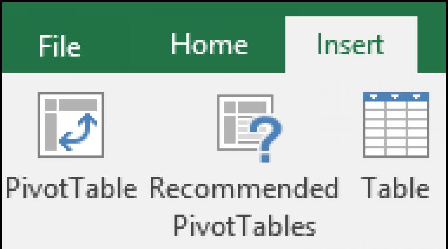
In order to directly start creating a pivot table, go to the "Insert" tab. Having passed, we click on the very first button in the ribbon, which is called “Pivot Table”. After that, a menu opens in which you should choose what we are going to create, a table or a chart. Click on the "Pivot Table" button.

A window opens in which we again need to select a range, or a table name. As you can see, the program has already pulled up the name of our table itself, so there is nothing more to do here. At the bottom of the dialog box, you can choose where the pivot table will be created: on a new sheet (by default), or on the same one. Of course, in most cases, it is much more convenient to use a pivot table on a separate sheet. But, this is an individual matter for each user, which depends on his preferences and tasks. We just click on the "OK" button.

After that, a form for creating a pivot table opens on a new sheet.

As you can see, in the right part of the window there is a list of table fields, and below are four areas:
- Row names;
- Column names;
- Values;
- Report filter.
Simply, we drag the table fields we need with the mouse to the areas that correspond to our needs. There is no clear set rule for which fields to move, because everything depends on the source table, and on specific tasks that can change.

So, in this particular case, we have moved the “Gender” and “Date” fields to the “Report Filter” area, the “Personnel Category” field to the “Column Names” area, the “Name” field to the “Row Names” area, the “Amount wages" in the "Values" area. It should be noted that all arithmetic calculations of data pulled from another table are possible only in the last area. As you can see, while we were doing these manipulations with the transfer of fields to areas, the table itself on the left side of the window changed accordingly.

Here is a pivot table. Filters by gender and date are displayed above the table.

PivotTable Setup
But, as we remember, only data for the third quarter should remain in the table. In the meantime, data for the entire period is displayed. In order to bring the table to the form we need, click on the button next to the "Date" filter. In the window that appears, check the box next to the inscription "Select multiple elements." Next, uncheck all dates that do not fit into the period of the third quarter. In our case, this is just one date. Click on the "OK" button.

In the same way, we can use the gender filter, and select only one male for the report, for example.

After that, the pivot table took on this form.

To demonstrate that you can manipulate the data in the table in any way, we reopen the field list form. To do this, go to the "Parameters" tab, and click on the "List of fields" button. Then, we move the “Date” field from the “Report Filter” area to the “Line Names” area, and between the “Personnel Category” and “Gender” fields, we exchange areas. All operations are performed using a simple drag and drop of elements.

Now, the table has a completely different look. Columns are divided by gender, rows now have a breakdown by month, and you can now filter the table by personnel category.

If in the list of fields the names of the lines are moved, and the date is put higher than the name, then it is the dates of payments that will be divided into the names of employees.

Also, you can display the numerical values of the table as a histogram. To do this, select a cell with a numerical value in the table, go to the "Home" tab, click on the " Conditional Formatting”, go to the “Histograms” item, and select the type of histogram you like.

As you can see, the histogram appears in only one cell. In order to apply the histogram rule for all cells of the table, click on the button that appeared next to the histogram, and in the window that opens, move the switch to the “To all cells” position.

Now, our pivot table has acquired a presentable look.

Creating a PivotTable Using the PivotTable Wizard
You can create a pivot table using the PivotTable Wizard. But, for this you need to immediately withdraw this instrument per panel quick access.Go to the "File" menu item, and click on the "Options" button.

In the options window that opens, go to the "Quick Access Panel" section. Select commands from the commands on the ribbon. In the list of elements, look for "PivotTable and PivotChart Wizard". Select it, click on the "Add" button, and then on the "OK" button in the lower right corner of the window.

As you can see, after our actions, a new icon has appeared on the Quick Access Toolbar. We click on it.

This will open the PivotTable Wizard. As you can see, we have four options for the data source from which the pivot table will be formed:
- in a list or database Microsoft data excel;
- in an external data source (another file);
- in several consolidation ranges;
- in another PivotTable or PivotChart.
At the bottom, you should choose what we are going to create, a pivot table or a chart. Make a choice and click on the "Next" button.

After that, a window appears with the range of the data table, which, if desired, can be changed, but we do not need to do this. Just click on the "Next" button.

Then, the PivotTable Wizard prompts you to choose a place where the new table will be placed on the same sheet or on a new one. We make a choice, and click on the "Finish" button.

After that, it opens new leaf with exactly the same form that opened with the usual way to create a pivot table. Therefore, it makes no sense to dwell on it separately.
All further actions are performed according to the same algorithm that was described above.
As you can see, create a pivot table in Microsoft program Excel can be done in two ways: in the usual way through the button on the ribbon, and using the PivotTable Wizard. The second method provides more additional features, but in most cases, the functionality of the first option is quite enough to complete the tasks. Pivot tables can form data into reports according to almost any criteria that the user specifies in the settings.
Excel PivotTables are one of the tools that help you quickly and easily analyze large amounts of information. We will show with examples how to build pivot tables in Excel.
In this article you will learn:
What is a PivotTable in Excel?
When working with data in Excel, periodically there is a need to analyze them. This is important, for example, in sales - who, in what period, how many made sales, when there was a recession, and when there was a surge, which goods are in the greatest demand, which are the least. The more data, the more difficult it is to analyze them. The higher the probability of error due to the human factor. Therefore, it is necessary to apply the tools that are provided by Excel itself.
Pivot tables MS Excel is a tool for analytics and data presentation in a convenient and easily understandable form. They are used in the following cases:
- Large amount of initial data. A small amount of data can be calculated and analyzed manually. However, if there are hundreds and thousands of records at your disposal, errors are inevitable and there will be many of them. The time required for processing will also increase significantly.
- It is necessary to identify trends and dynamics in the data. In pivot tables, you can easily transform the output of information, you do not need to sort it manually.
- To create a chart or graph based on formatted data.
- It is necessary to make an intermediate "cut" of the results, which often change, for their subsequent comparison. In this case, it is enough to update the data, Excel will recalculate everything automatically.
- For analysis and search for extreme values - data minima and maxima.
- To bring together disparate data from different sources. If necessary, you can add the required row or column to the source data and update the final display of the report.
Also, pivot tables in Excel are more convenient to use when viewing data. .
What does a pivot table look like
Before we talk about how to build a pivot table in Excel, let's show how it looks. The data for the table is taken from the user-specified shared table. Functionally, the table is divided into four segments:
- values;
- lines;
- columns;
- report filter.
The PivotTable of the .xlsx file has the following limitations:
- the maximum number of row fields is 1,048,576 or limited by the size of the RAM;
- the maximum number of column fields is 16,384;
- the maximum number of page fields is 16,384;
- the maximum number of data fields is 16,384.
Let's take the following data as an example.
The pivot table for this data will look like this:

In the right part of the pivot table - last names, at the top - dates, in the center - the results of the work. Obviously, this presentation of information is more convenient and understandable. .

In this image, the value segment is highlighted in red. This is the segment in which the calculations are carried out. Here you can see the cost of concluded deals by day and by last name.

This is a string segment. There may be one or more values here. In our case, these are the names of managers. Opposite the names in the corresponding lines - a summary of the work.

This is the column segment. Usually it is a time scale, its use facilitates the analysis and perception of data.
In a special pivot table wizard, you can change the placement of data. In our case, last names can be placed in the column segment, in dates - in the row segment. Then the pivot table will take on a new look.

The PivotTable Builder is intuitive. In it, you can drag values into fields, you can select values from a drop-down list. Further in the article, a tutorial on creating a pivot table in Excel with examples. .
How to Create a PivotTable in Excel
We will tell and show with examples how to create a pivot table in Excel. As initial data, let's take our table with information on the work of managers for May. To create a pivot table, you need to top menu In the "Insert" tab, select "Pivot Table". They are highlighted in the picture.

A new window will appear:

It will need to specify the source whose data will be used to build the pivot table. To do this, you need to select the desired area or the entire table and Excel will substitute this data in a row.

The color shows that the entire array is selected, data appeared in the line. You then need to specify where Excel should build the pivot table. You can select the current sheet or select a new sheet.
If you select a new sheet, then in this case it will be created, the pivot table designer will appear on it. We recommend doing so. After all the information is specified - the source data and the place for the report, you must click the "OK" button and a prompt will appear prompting you to select the fields for building a new report.

To the right of it, a section will open in which you can specify the fields to add them to the pivot table.

Under it there will be another work field where you can drag fields to different areas.

You need to check the boxes for the required fields. The specified positions will automatically appear in the bottom section. They can be customized to your liking.

When rebuilding the source data, the display will be automatically rebuilt. If there are many values, then this can interfere with normal operation. Therefore, you can check the "Defer layout update" checkbox. Automatic rebuilding will be disabled. To refresh the pivot table, just click the Refresh button.

Thus, we will create a pivot table and it will take the following form.

It can be seen that the order of the lines matters. The first line in the constructor comes first. The second line in the constructor becomes a subparagraph of the first. In our case, the results of the work of each manager are shown with a breakdown by commodity items - articles with reference to dates.
You can change the order of the lines - to do this, just drag the desired line up or down with the mouse. If you swap the surname and article, then the pivot table will take the following form.

For ease of perception of information, sub-items can be collapsed. By default, they are displayed expanded. To collapse unnecessary positions, you must click the minus sign next to the article. Then the sub-items will be hidden. To expand them, click the plus sign. They are highlighted in the picture.

The central value segment will display all the information summarized and calculated by the program. The total will also be shown - by dates, by articles, and if the article is not collapsed - then by the names of managers.
If you make changes to the original table, the pivot table must be updated. To do this, right-click anywhere in its place and select in the appeared context menu"Update". The data will be rebuilt.

If new rows or columns have been added and the old report display does not cover all the required data set, you must include them in the pivot table. For example, new data has been added to the main array of information (highlighted in color) and the pivot table does not take them into account yet.

To add them to the report, you need to click on the pivot table, go to the "Parameters" tab and select "Change data source" - this option is highlighted in the picture.
In the window that appears, specify the data source along with the updated rows and click OK.

The pivot table will automatically rebuild. On the image, the data for 05/29/2018, which were not available earlier, are highlighted in color.

VIDEO: How to work with pivot tables
This part of the tutorial details how to create a PivotTable in Excel. This article was written for Excel 2007 (as well as later versions). Instructions for more early versions Excel can be found in a separate article: How to create a PivotTable in Excel 2003?
As an example, consider the following table, which contains a company's sales data for the first quarter of 2016:
| A | B | C | D | E | |
|---|---|---|---|---|---|
| 1 | Date | Invoice Ref | Amount | Sales Rep. | region |
| 2 | 01/01/2016 | 2016-0001 | $819 | Barnes | North |
| 3 | 01/01/2016 | 2016-0002 | $456 | Brown | South |
| 4 | 01/01/2016 | 2016-0003 | $538 | Jones | South |
| 5 | 01/01/2016 | 2016-0004 | $1,009 | Barnes | North |
| 6 | 01/02/2016 | 2016-0005 | $486 | Jones | South |
| 7 | 01/02/2016 | 2016-0006 | $948 | Smith | North |
| 8 | 01/02/2016 | 2016-0007 | $740 | Barnes | North |
| 9 | 01/03/2016 | 2016-0008 | $543 | Smith | North |
| 10 | 01/03/2016 | 2016-0009 | $820 | Brown | South |
| 11 | … | … | … | … | … |
To begin with, let's create a very simple pivot table that will show the total sales of each of the sellers according to the table above. To do this, do the following:
The PivotTable will be populated with the sales totals for each salesperson, as shown in the image above.
If you want to display sales volumes in monetary units, you must format the cells that contain these values. The easiest way to do this is to highlight the cells whose format you want to customize and select the format Monetary(Currency) section Number(Number) tab home(Home) Excel menu ribbons (as shown below).

As a result, the pivot table will look like this:

Please note that the default currency format depends on the system settings.
IN latest versions Excel (Excel 2013 or later) tab Insert(Insert) button present Recommended pivot tables(Recommended Pivot Tables). Based on the selected source data, this tool suggests possible pivot table formats. Examples can be viewed at
Pivot tables in Excel are a powerful reporting tool. It is especially useful in cases where the user does not work well with formulas and it is difficult for him to do data analysis on his own. In this article, we will look at how to create such tables correctly and what opportunities exist for this in the Excel editor. You don't need to download any files for this. Training is available online.
The first step is to create a table. It is desirable that there are several columns. In this case, some information must be repeated, since only in this case it will be possible to make some analysis of the entered information.
For example, consider the same financial expenses in different months.

Creating pivot tables
In order to build such a table, you need to do the following steps.
- To begin with, it must be completely selected.

- Then go to the "Insert" tab. Click on the "Table" icon. Select "Pivot Table" from the menu that appears.

- As a result of this, a window will appear in which you need to specify several basic parameters for building a pivot table. The first step is to select the data area on the basis of which the analysis will be carried out. If you have previously selected a table, then a link to it will be inserted automatically. Otherwise, it will need to be selected.

- You will then be asked to specify exactly where the build will take place. It is better to select the item “To an existing sheet”, since it will be inconvenient to analyze information when everything is scattered over several sheets. Then you need to specify the range. To do this, click on the icon next to the input field.

- Immediately after that, the PivotTable Wizard will collapse to a small size. In addition, it will also change appearance cursor. You will need to make a left mouse click in any place convenient for you.

- As a result, the reference to the specified cell will be substituted automatically. Then you need to click on the icon on the right side of the window to restore it to its original size.

- To complete the settings, click on the "OK" button.

- As a result of this you will see blank template, to work with pivot tables.

- At this stage, you need to specify which field will be:
- column;
- string;
- value for analysis.
You can choose anything. It all depends on what kind of information you want to receive.

- In order to add any field, you need to left-click on it and, without releasing your finger, drag it to the desired area. The cursor will change its appearance.

- You can release your finger only when the crossed out circle disappears. Similarly, you need to drag all the fields that are in your table.

- To see the whole result, you can close the settings sidebar. To do this, just click on the cross.

- As a result of this, you will see the following. With this tool, you will be able to summarize the amount of expenses in each month for each item. In addition, information about the total result is available.

- If you don't like the table, you can try building it a little differently. To do this, you need to change the fields in the construction areas.

- Close the build assistant again.

- This time, we can see that the PivotTable has become much larger, since now the columns are not months, but categories of expenses.

If you are unable to build a table yourself, you can always count on the help of an editor. In Excel, it is possible to create similar objects in automatic mode.
To do this, you must do the following, but first select all the information in its entirety.

- Go to the "Insert" tab. Then click on the "Table" icon. In the menu that appears, select the second item.

- Immediately after that, a window will appear in which there will be various examples for building. Similar options are suggested based on multiple columns. The number of templates directly depends on their number.

- When hovering over each item, a preview of the result will be available. This makes it much more convenient to work.

- You can choose what you like the most.

- To insert the selected option, just click on the "OK" button.

- As a result, you will get the following result.

Note that the table has been created on a new sheet. This will happen every time the constructor is used.
As soon as you add (no matter how) a pivot table, you will see on the toolbar new tab"Analysis". It contains a huge number of different tools and functions.

Let's consider each of them in more detail.
By clicking on the button marked in the screenshot, you can do the following:
- change name;

- bring up the settings window.

In the options window you will see a lot of interesting things.

active field
With this tool, you can do the following:
- First you need to select a cell. Then click on the "Active field" button. In the menu that appears, click on the "Field Options" item.

- Right after that, you will see the following window. Here you can specify the type of operation that should be used to summarize the data in the selected field.

- In addition, you can set number format. To do this, click on the appropriate button.

- This will bring up the Format Cells window.

Here you can specify in what form you want to display the result of the analysis of information.
Thanks to this tool, you can customize grouping by selected values.

Paste Slice
The Microsoft Excel editor allows you to create interactive pivot tables. In this case, you do not need to do anything complicated.
- Select a column. Then click on the "Insert Slice" button.
- In the window that appears, as an example, select one of the proposed fields (in the future, you can select them in an unlimited number). After something is selected, the "OK" button is immediately activated. Click on it.

- As a result, a small window will appear that can be moved anywhere. It will offer all possible unique values that are in this field. Thanks to this tool, you will be able to withdraw the amount only for certain months (in this case). By default, information is displayed for all time.

- You can click on any of the items. Immediately after that, all values in the sum field will change.

- Thus, it will be possible to choose any period of time.

- At any time, everything can be returned to its original form. To do this, click on the icon on the right upper corner this window.

In this case, we were able to sort the report by month because we had the corresponding field. But there is a more powerful tool for working with dates.
If you click on the corresponding button on the toolbar, you will most likely see this error. The fact is that in our table there are no cells that will have the "Date" data format explicitly.

As an example, let's create a small table with various dates.

Then you will need to build a pivot table.
Go back to the "Insert" tab. Click on the "Table" icon. In the submenu that appears, select the option we need.

- We are then asked to select a range of values.

- To do this, it is enough to select the entire table.

- Immediately after that, the address will be substituted automatically. Everything is very simple here, because it is designed for dummies. Click the OK button to complete the build.

- The Excel editor will offer us only one option, since the table is very simple (no more is needed for the example).

- Try clicking the "Insert Timeline" icon again (located on the "Analysis" tab).

- This time there will be no errors. You will be prompted to select a field for sorting. Check the box and click the OK button.

- Thanks to this, a window will appear in which you can select the desired date using the slider.

- We choose another month and there is no data, since all expenses in the table are indicated only for March.

If you have made any changes to the original data and for some reason this is not displayed in the pivot table, you can always update it manually. To do this, just click on the corresponding button on the toolbar.

If you decide to change the fields on which the building should be based, then it is much easier to do this in the settings, rather than deleting the table and creating it again taking into account new preferences.
To do this, click on the "Data Source" icon. Then select the menu item of the same name.

As a result of this, a window will appear in which you can re-select the required amount of information.

Actions
With this tool you will be able to:
- clear the table;
- highlight;
- move it.

Computing
If the calculations in the table are not enough or they do not meet your needs, you can always make your own changes. By clicking on the icon of this tool, you will see the following options.

These include:
- calculated field;

- computed object;

- calculation order (added formulas are displayed in the list);

- display formulas (no information, as there are no added formulas).

Here you can create a PivotChart or change the recommended table type.

With this tool, you can customize the appearance of the editor workspace.

Thanks to this, you will be able to:
- customize the display of the sidebar with a list of fields;

- enable or disable the plus/minus buttons;

- customize the display of field headers.

When working with pivot tables, in addition to the "Analysis" tab, another one will also appear - "Designer". Here you can change the appearance of your object until it is unrecognizable compared to the default.

Can be customized:
- subtotals:
- do not show;
- show all totals at the bottom;
- show all totals in header.

- overall results:
- disable for rows and columns;
- enable for rows and columns;
- enable for rows only;
- enable for columns only.

- report layout:
- show in a condensed form;
- show in structure form;
- show in tabular form;
- repeat all element labels;
- do not repeat element labels.

- empty lines:
- insert a blank line after each element;
- remove empty line after each element.

- PivotTable style options (here you can enable/disable each item):
- line headers;
- column headings;
- alternating lines;
- alternating columns.

- customize the style of the elements.

In order to see more different options, you need to click on the triangle in the lower right corner of this tool.

Immediately after that, a huge list will appear. You can choose anything. When you hover over each of the templates, your table will change (this is done for preview). Changes will not take effect until you click on any of the options.

In addition, if you wish, you can create your own design style.

You can also change the order in which rows are displayed here. Sometimes this is necessary for the convenience of cost analysis. Especially if the list is very large, since the required position is easier to find alphabetically than scrolling through the list several times.
To do this, do the following.
- Click on the triangle next to the required field.
- As a result, you will see the following menu. Here you can select the desired sorting option ("A to Z" or "Z to A").

If the standard option is not enough, you can click on the item " Extra options sorting".

As a result, you will see the following window. For more detailed settings you need to click on the "Advanced" button.

Everything here is set to automatic. If you clear this checkbox, you can specify the key you need.

Pivot Tables in Excel 2003
The steps above are suitable for modern editors (2007, 2010, 2013 and 2016). IN old version everything looks different. Opportunities, of course, there are much less.
In order to create a pivot table in Excel 2003, you need to do the following.
- Go to the "Data" menu section and select the appropriate item.

- As a result, a wizard for creating such objects will appear.

- After clicking on the "Next" button, a window will open in which you need to specify a range of cells. Then click on "Next" again.

- To complete the settings, click on "Finish".

- As a result of this, you will see the following. Here you need to drag the fields to the appropriate areas.

- For example, you might get the following result.

It becomes obvious that it is much better to create such reports in modern editors.
Conclusion
This article covered all the subtleties of working with pivot tables in the Excel editor. If something doesn't work out for you, you may select the wrong fields or there are very few of them - to create such an object, you need several columns with duplicate values.
If this tutorial you are not enough Additional information can be found in Microsoft's online help.
Video instruction
For those who still have unanswered questions, a video with comments on the instructions described above is attached below.