How to make a formula in xl table. Formulas in Excel

For most users, Excel is a program that can work with tables and in which you can put the relevant information in a tabular form. As a rule, few people know all the possibilities of this program, and it is unlikely that anyone thought much about it. And Excel can do a large number of operations, and one of them is to count numbers.

Simple operations in MS Excel

To the program Microsoft Excel as if an ultra-modern calculator is built in with big amount functions and features.
So, the first thing you need to know is that all calculations in Excel are called formulas and they all start with an equal sign (=). For example, you need to calculate the sum of 5 + 5. If you select any cell and write 5 + 5 inside it, and then press the Enter button, the program will not calculate anything - the cell will simply say “5 + 5”. But if we put an equal sign (=5+5) in front of this expression, then Excel will give us the result, that is, 10.

You also need to know the basic arithmetic operators to work in Excel. These are the standard functions: addition, subtraction, multiplication and division. Excel also offers exponentiation and percentage. With the first four functions, everything is clear. Exponentiation is written as ^ (Shift+6). For example, 5^2 would be five squared, or five raised to the second power.
As for the percentage, if you put a% sign after any number, it will be divisible by 100. For example, if you write 12%, you get 0.12. With this sign it is easy to calculate percentages. For example, if you need to calculate 7 percent out of 50, then the formula will look like this: \u003d 50 * 7%.

One of the popular operations that is often done in Excel is the sum calculation. Suppose there is a table with the fields "Name", "Quantity", "Price" and "Amount". All of them are filled in, only the "Amount" field is empty. To calculate the sum and automatically fill in the free column, you first need to select the cell where you want to write the formula, and put an equal sign. Then click on the desired number in the "Quantity" field, type the multiplication sign, then click on the number in the "Price" field and press Enter. The program will calculate this expression. If you click on the sum cell, you can see something like this formula: \u003d B2 * C2. This means that not some specific numbers were counted, but the numbers that were in these cells. If you write other numbers in the same cells, Excel will automatically recalculate the formula - and the value of the sum will change.

If you need, for example, to count the number of all goods that are recorded in the table, this can be done by selecting the autosum icon in the toolbar (it looks like the letter E). After that, you will need to specify the range of cells that you want to count (in this case, all the numbers in the "Quantity" field), press Enter - and the program will display the resulting value. You can also do this manually by specifying all the cells of the "Quantity" field one by one and putting an addition sign between them. (=A1+A2+…A10). The result will be the same.

Excel is designed to work with tabular data and make calculations using formulas of various levels of complexity. Calculating the sum over a column or row, over several ranges of values ​​​​at once is an easy task if you know how to do it correctly.

Method 1 - AutoSum

This action allows you to quickly find out the total for a column without the skills of creating formulas. Action algorithm:

If you want to sum several columns or rows at once, then:


If you want to find the sum along with several additional cells:

Method 2. Manual formula entry

It is convenient, if necessary, to calculate the sum of the addition of values ​​that are randomly located in relation to each other. Create a formula step by step:

Method 3. Visual summation

The peculiarity of this method is that the total is not displayed in a separate cell, there is no need to use formulas. The end result will be visible in the lower right corner of the document sheet with the range of cells selected. As soon as the selection is removed, the amount disappears. Step by step:


Examples were considered on columns, a similar sequence of actions when summing values ​​in rows. The difference is that the range is selected not vertically, but horizontally.

Hello!

Many who do not use Excel - do not even imagine what opportunities this program gives! Just think: put in automatic mode values ​​from one formula to another, search for the desired lines in the text, add by condition, etc. - in general, in fact, a mini-programming language for solving "narrow" tasks (to be honest, I myself have long excel time did not consider it for the program, and almost did not use it) ...

In this article I want to show a few examples of how you can quickly solve everyday office tasks: add something, subtract something, calculate the sum (including with a condition), substitute values ​​from one table to another, etc. That is, this article will be something like a mini guide on learning the most necessary things for work (more precisely, to start using Excel and feel the full power of this product!).

It is possible that if you had read a similar article 15-17 years ago, I myself would have started using Excel much faster (and would have saved a lot of my time for solving "simple" (note: as I understand now) tasks)...

Note: All screenshots below are from Excel 2016 (as the newest to date).

Many novice users, after starting Excel, ask one strange question: "well, where is the table?". Meanwhile, all the cells that you see after starting the program are one big table!

Now to the main thing: in any cell there can be text, some number, or a formula. For example, the screenshot below shows one illustrative example:

• left: Cell (A1) contains the prime number "6". Note that when you select this cell, the formula bar (Fx) just shows the number "6".
• right : in cell (C1) it also looks like a simple number "6", but if you select this cell, you will see the formula "=3+3" - this is an important feature in Excel!

Just a number (on the left) and a calculated formula (on the right)

The bottom line is that Excel can count like a calculator if you select some cell, and then write a formula, for example "=3+5+8" (without quotes). You do not need to write the result - Excel will calculate it and display it in the cell (as in cell C1 in the example above)!

But you can write in formulas and add not just numbers, but also numbers already calculated in other cells. In the screenshot below, in cell A1 and B1, the numbers are 5 and 6, respectively. In cell D1, I want to get their sum - you can write the formula in two ways:

• first: "=5+6" (not very convenient, imagine that in cell A1 - we also have a number calculated according to some other formula and it changes. You won’t substitute a number instead of 5 every time?!);
• the second: "=A1+B1" - and this is the ideal option, just add the value of cells A1 and B1 (regardless of what numbers they contain!)

Add cells that already have numbers

Extending a formula to other cells

In the example above, we added two numbers in column A and B in the first row. But then we have 6 lines, and most often in real problems you need to add numbers in each line! To do this, you can:

1. on line 2 write the formula "=A2+B2" , on line 3 - "=A3+B3", etc. (this is long and tedious, this option is never used);
2. select cell D1 (which already has a formula), then move the mouse pointer to the right corner of the cell so that a black cross appears (see screenshot below). Then hold down the left button and stretch the formula to the entire column. Convenient and fast! (Note: You can also use Ctrl+C and Ctrl+V combinations for formulas (copy and paste respectively)).

By the way, pay attention to the fact that Excel itself has substituted formulas in each line. That is, if you now select a cell, say D2, you will see the formula "=A2+B2" (i.e. Excel automatically fills in the formulas and returns the result immediately) .

How to set a constant (a cell that will not change when copying a formula)

Quite often it is required in formulas (when you copy them) that some value does not change. Let's say a simple task: convert prices in dollars into rubles. The cost of the ruble is set in one cell, in my example below it is G2.

Next, in cell E2, the formula "=D2*G2" is written and we get the result. Only now, if we stretch the formula, as we did before, we will not see the result in other lines, because Excel in line 3 will put the formula "D3*G3", in the 4th line: "D4*G4", etc. G2 must remain G2 everywhere...

To do this - just change cell E2 - the formula will look like "=D2*$G$2". Those. dollar sign $ - allows you to set a cell that will not change when you copy the formula (i.e. get a constant, example below)...

How to calculate the sum (SUM and SUMIFS formulas)

You can, of course, write formulas in manual mode, typing "=A1+B1+C1" and so on. But Excel has faster and more convenient tools.

One of the most simple ways add all selected cells is to use the option autosums (Excel will write the formula itself and paste it into the cell).

1. first select the cells (see screenshot below);
2. then open the section "Formulas";
3. The next step is to press the "Autosum" button. Under the cells you selected, the result of the addition will appear;
4. if you select the cell with the result (in my case, this is the cell E8) - then you will see the formula "=SUM(E2:E7)" .
5. thus writing the formula "=SUM(xx)", where instead of xx put (or select) any cells, you can read a wide variety of ranges of cells, columns, rows...

Quite often, when working, it is required not just the sum of the entire column, but the sum of certain rows (i.e. selectively). Suppose a simple task: you need to get the amount of profit from some worker (exaggerated, of course, but the example is more than real).

I will use only 7 rows in my table (for clarity), the real table can be much larger. Suppose we need to calculate all the profit that "Sasha" made. What the formula will look like:

1. "=SUMIFS(F2:F7 ;A2:A7 ;"Sasha") " - (note: pay attention to the quotation marks for the condition - they should be like in the screenshot below, and not as it is written on my blog now). Also note that Excel, when driving in the beginning of a formula (for example, "SUM ..."), itself prompts and substitutes possible options - and there are hundreds of formulas in Excel!;
2. F2:F7 - this is the range over which the numbers from the cells will be added (summed up);
3. A2:A7 is the column by which our condition will be checked;
4. "Sasha" is a condition, those lines in which "Sasha" will be in column A will be added (pay attention to the indicative screenshot below).

Note: there can be several conditions and you can check them in different columns.

How to count the number of rows (with one, two or more conditions)

Quite a typical task: to calculate not the sum in the cells, but the number of rows that satisfy some condition. Well, for example, how many times the name "Sasha" occurs in the table below (see screenshot). Obviously, 2 times (but this is because the table is too small and taken as a good example). How can this be calculated as a formula? Formula:

"=COUNTIF(A2:A7 ,A2 )" - Where:

• A2:A7- the range in which lines will be checked and counted;
• A2- a condition is set (note that you could write a condition like "Sasha", or you can just specify a cell).

The result is shown on the right side of the screenshot below.

Now imagine a more extended task: you need to count the lines where the name "Sasha" occurs, and where in the AND column there will be the number "6". Looking ahead, I will say that there is only one such line (screen with an example below).

The formula will look like:

=COUNTIFS(A2:A7 ;A2 ;B2:B7 ;"6") (note: pay attention to the quotes - they should be like in the screenshot below, and not like mine), Where:

A2:A7 ;A2- the first range and search condition (similar to the example above);

B2:B7 ;"6"- the second range and the search condition (note that the condition can be specified in different ways: either specify a cell, or simply write text/number in quotes).

How to calculate the percentage of the amount

It's a very common question that I often come across. In general, as far as I can imagine, it occurs most often - due to the fact that people get confused and do not know what percentage is looking for (and in general, they do not understand the topic of interest well (although I myself am not a great mathematician, and yet ...)).

The simplest way, in which it is simply impossible to get confused, is to use the "square" rule, or proportion. The whole essence is shown on the screen below: if you have a total amount, let's say in my example this number is 3060 - cell F8 (i.e. this is 100% profit, and "Sasha" made some part of it, you need to find which ... ).

In proportion, the formula will look like this: =F10*G8/F8(i.e. cross by cross: first we multiply two known numbers diagonally, and then divide by the remaining third number). In principle, using this rule, it is almost impossible to get lost in percentages.

Actually, this concludes this article. I'm not afraid to say that having mastered everything that is written above (and only "heels" of formulas are given here) - you will be able to learn Excel on your own, flip through help, watch, experiment, and analyze. I will say even more, everything that I described above will cover many tasks, and will allow you to solve the most common ones that you often puzzle over (if you don’t know the capabilities of Excel), and you don’t know how to do it faster ...

Microsoft Excel is not only a large spreadsheet, but also an ultra-modern calculator with many features and capabilities. In this lesson, we will learn how to use it for its intended purpose.

All calculations in Excel are called formulas, and they all start with an equal sign (=).

For example, I want to calculate the sum of 3+2. If I click on any cell and type 3+2 inside, and then press the Enter button on the keyboard, then nothing will be calculated - 3+2 will be written in the cell. But if I type =3+2 and press Enter, then everything will be calculated and the result will be shown.

Remember two rules:

All calculations in Excel start with =

After entering the formula, you need to press the Enter button on the keyboard

And now about the signs with which we will count. They are also called arithmetic operators:

Addition

Subtraction

* multiplication

/ division. There is also a stick with an inclination to the other side. Well, it doesn't suit us.

^ exponentiation. For example, 3^2 is read as three squared (to the second power).

% percent. If we put this sign after any number, then it is divisible by 100. For example, 5% will be 0.05.
This symbol can be used to calculate percentages. If we need to calculate five percent out of twenty, then the formula will look like this: \u003d 20 * 5%

All these signs are on the keyboard either at the top (above the letters, along with numbers), or on the right (in a separate block of buttons).

To print characters at the top of the keyboard, you need to press and hold the button labeled Shift and, together with it, press the button with the desired character.

Now let's try to count. Let's say we need to add the number 122596 to the number 14830. To do this, left-click on any cell. As I said, all calculations in Excel begin with the "=" sign. So, in the cell you need to print = 122596 + 14830

And in order to get the answer, you need to press the Enter button on the keyboard. After that, the cell will no longer have a formula, but a result.

And now pay attention to this top field in the Excel program:

This is the Formula Bar. We need it in order to check and change our formulas.

For example, click on the cell in which we just calculated the amount.

And look at the formula bar. It will show exactly how we got this value.

That is, in the formula bar we see not the number itself, but the formula with which this number was obtained.

Try to type the number 5 in some other cell and press Enter on the keyboard. Then click on that cell and look in the formula bar.

Since we simply typed this number, and did not calculate it using a formula, it will only be in the formula bar.

How to count correctly

But, as a rule, this method of "counting" is not used so often. There is a more advanced version.

Let's say we have a table like this:

I'll start with the first position "Cheese". I click in cell D2 and type an equal sign.

Then I click on cell B2, since I need to multiply its value by C2.

I print the multiplication sign *.

Now I click on cell C2.

And finally, I press the Enter button on the keyboard. All! Cell D2 has the desired result.

By clicking on this cell (D2) and looking in the formula bar, you can see how this value was obtained.

Let me explain using this table as an example. Now the number 213 is entered in cell B2. I delete it, type another number and press Enter.

Let's look at the cell with the sum D2.

The result has changed. This happened because the value in B2 changed. After all, we have the following formula: \u003d B2 * C2

It means that Microsoft program Excel multiplies the contents of cell B2 by the contents of cell C2, whatever it is. Draw your own conclusions :)

Try to make the same table and calculate the sum in the remaining cells (D3, D4, D5).

Over the past decade, the computer in accounting has become simply an indispensable tool. At the same time, its application is diverse. The first is, of course, the use accounting program. To date, quite a few have been developed software tools, both specialized ("1C", "Info-Accountant", "BEST", etc.), and universal, like Microsoft Office. At work, and in everyday life, you often have to do a lot of different calculations, keep multi-line tables with numerical and text information, doing all sorts of calculations with the data, printing options. To solve a number of economic and financial problems, it is advisable to use the numerous possibilities of spreadsheets. Consider in this connection the computational functions of MS Excel.

Vladimir SEROV, PhD, Olga TITOVA

Source: Journal "Accountant and Computer" No. 4, 2004.

Like any other spreadsheet, MS Excel is designed primarily to automate calculations that are usually made on a piece of paper or using a calculator. In practice, in professional activities there are quite complex calculations. That's why we'll take a closer look at how Excel helps us automate their execution.

Operators are used in formulas to indicate an action, such as addition, subtraction, etc.

All operators are divided into several groups (see table).

OPERATOR	MEANING	EXAMPLE
ARITHMETIC OPERATORS
+ (plus sign)	Addition	=A1+B2
- (minus sign)	Subtraction Unary minus	=A1-B2 =-B2
/(slash)	Division	=A1/B2
*(star)	Multiplication	= A1*B2
% (percent sign)	Percent	=20%
^ (cap)	Exponentiation	= 5^3 (5 to the 3rd power)
COMPARISON OPERATORS
=	Equals	=IF(A1=B2,"Yes","No")
>	More	=IF(A1>B2,A1,B2)
<	Less	=IF(AKV2,B2,A1)
>= <=	Greater than or equal Less than or equal	=IF(A1>=B2,A1,B2) =IF(AK=B2,B2,A1)
<>	Not equal	=IF(A1<>B2; "Not Equal")
TEXT OPERATOR
&(ampersand)	Combining character sequences into a single character sequence	= "The value of cell B2 is: "&B2
ADDRESS OPERATORS
Range(colon)	Referencing all cells between the bounds of a range, inclusive	=SUM(A1:B2)
Concatenation (semicolon)	Link to merge range cells	=SUM(A1:B2,SZ,D4:E5)
Intersection(space)	Link to shared range cells	=CUMM(A1:B2C3D4:E5)

Arithmetic operators are used to denote basic mathematical operations on numbers. The result of the execution arithmetic operation is always a number. Comparison operators are used to denote the operations of comparing two numbers. The result of the comparison operation is the logical value TRUE or FALSE.

Formulas are used to perform calculations in Excel. Using formulas, you can, for example, add, multiply, and compare table data, i.e., formulas should be used when you need to enter a calculated value into a sheet cell (automatically calculate). Entering a formula begins with the symbol “=” (equal sign). It is this sign that distinguishes the input of formulas from the input of text or a simple numeric value.

When entering formulas, you can use regular numeric and text values. Recall that numeric values ​​can only contain numbers from 0 to 9 and Special symbols: (plus, minus, slash, round brackets, dot, comma, percent and dollar signs). Text values can contain any characters. It should be noted that text expressions used in formulas must be enclosed in double quotes, for example “constant1”. In addition, in formulas, you can use cell references (including in the form of names) and numerous functions that are interconnected by operators.

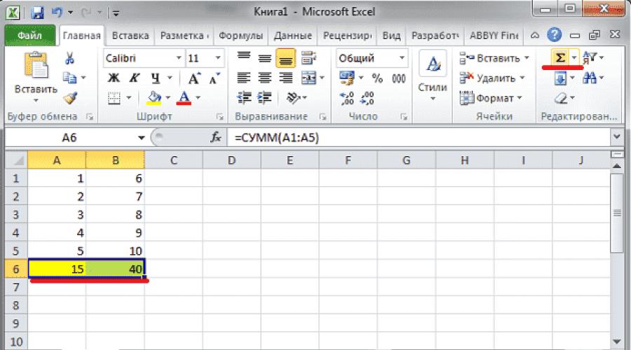
References are cell addresses or ranges of cells included in a formula. Cell references are set in the usual way, that is, in the form A1, B1, C1. For example, in order to get the sum of cells A1 and A2 in cell A3, it is enough to enter the formula =A1+A2 into it (Fig. 1).

When entering a formula, cell references can be typed character by character directly from the Latin keyboard, but more often it is much easier to specify them with the mouse. For example, to enter the formula =A1+B2, you would do the following:

Select the cell in which you want to enter the formula;

Start entering the formula by pressing the “=” (equals) key;

Click on cell A1;

Enter the “+” symbol;

Click on cell B2;

Finish entering the formula by pressing the Enter key.

A cell range is a certain rectangular area of ​​a worksheet and is uniquely defined by cell addresses located in opposite corners of the range. Separated by “:” (colon), these two coordinates make up the address of the range. For example, to get the sum of cell values ​​in the range C3:D7, use the formula =SUM(C3:D7).

In the special case when a range consists entirely of several columns, for example from B to D, its address is written as B:D. Similarly, if the entire range consists of lines 6 through 15, then it has the address 6:15. In addition, when writing formulas, you can use the union of several ranges or cells, separating them with the symbol “;” (semicolon), for example C3:D7; E5;F3:G7.

Editing an already entered formula can be done in several ways:

Double-clicking the left mouse button on a cell to correct the formula directly in that cell;

Select a cell and press the F2 key (Fig. 2);

Select a cell by moving the cursor to the formula bar, click the left mouse button.

As a result, the program will enter the editing mode, during which you can make the necessary changes to the formula.

When filling out a table, it is customary to set calculation formulas only for the “first” (initial) row or “first” (initial) column, and fill the rest of the table with formulas using copy or fill modes. An excellent result is the use of autocopying formulas using an autofiller.

Recall how to correctly implement the copy mode. There may be various options (and problems too).

It must be borne in mind that when copying, the addresses are transposed. When you copy a formula from one cell to another, Excel reacts differently to formulas with relative and absolute references. For relative terms, Excel by default performs the transposition of addresses, depending on the position of the cell into which the formula is copied.

For example, you need to add row by row the values ​​of columns A and B (Fig. 8) and place the result in column C. If you copy the formula \u003d A2 + B2 from cell C2 to cell C3 * (and further down C), then Excel itself will convert formula addresses respectively as =A3+B3 (and so on). But if you need to put a formula, say, from C2 into cell D4, then the formula will already look like =B4+C4 (instead of the desired =A4+B4), and accordingly the calculation result will be wrong! In other words, pay special attention to the copying process and manually adjust the formulas if necessary. By the way, copying itself from C2 to C3 is done as follows:

1) select cell C2 from which you want to copy the formula;

2) press the “Copy” button on the toolbar, or the Ctrl+C keys, or select “Edit ® Copy” from the menu;

3) select cell C3, into which we will copy the formula;

4) press the “Paste” button on the toolbar, or the Ctrl + V keys, or through the menu “Edit ® Paste” with pressing Enter.

Consider the autocomplete mode. If you need to transfer (copy) the formula to several cells (for example, in C3:C5) down the column, then it is more convenient and easier to do this: repeat the previous sequence of actions until step 3 of selecting cell C3, then move the mouse cursor to the initial cell of the range ( C3), press the left mouse button and, without releasing it, drag it down to the required last cell of the range. In our case, this is cell C5. Then release the left mouse button, move the cursor to the “Insert” button on the toolbar and press it, and then Enter. Excel itself converts the addresses of the formulas in the range we have selected to the corresponding row addresses.

Sometimes it becomes necessary to copy only the numeric value of a cell (range of cells). To do this, do the following:

1) select a cell (range) from which you want to copy data;

2) click the “Copy” button on the toolbar or select “Edit ® Copy” from the menu;

3) select a cell (upper left of the new range) to which the data will be copied;

4) select in the menu “Edit ® Special insert” and press Enter.

When copying formulas, the computer immediately makes calculations on them, thus giving a quick and visual result.

:: Functions in Excel

Functions in Excel greatly facilitate calculations and interaction with spreadsheets. The most commonly used function is the summation of cell values. Recall that it has the name SUM, and the ranges of summed numbers serve as arguments.

In a spreadsheet, you often want to calculate a total for a column or row. To do this, Excel offers an automatic sum function, performed by clicking the button (“AutoSum”) on the toolbar.

If we enter a series of numbers, place the cursor under them and double-click on the auto-sum icon, then the numbers will be added (Fig. 3).

IN latest version program to the right of the autosum icon there is a list button that allows you to perform a number of frequently used operations instead of summing (Fig. 4).

:: Automatic calculations

Some calculations can be done without entering formulas at all. Let's make a small lyrical digression, which may be useful for many users. As you know, a spreadsheet, due to its user-friendly interface and computing capabilities can completely replace calculations using a calculator. However, practice shows that a significant part of people who actively use Excel in their activities keep a calculator on their desktop to perform intermediate calculations.

Indeed, in order to perform the operation of summing two or more cells in Excel to obtain a temporary result, you must perform at least two extra operations - find the place in the current table where the total will be located, and activate the autosum operation. And only after that you can select those cells whose values ​​need to be summed.

That's why, starting with Excel 7.0, the auto-calculate feature has been built into the spreadsheet. Excel spreadsheets now have the ability to fast execution some mathematical operations in automatic mode.

To see the result of intermediate summation, it is enough just to select the necessary cells. This result is also reflected in the status bar at the bottom of the screen. If the amount does not appear there, move the cursor to the status bar at the bottom of the frame, click right click mouse and in the drop-down menu near the Amount line, press the left mouse button. Moreover, in this menu on the status bar, you can select different options for the calculated results: the sum, the arithmetic mean, the number of elements, or the minimum value in the selected range.

For example, let's use this function to calculate the sum of values ​​for the range B3:B9. Select the numbers in the cell range B3:B9. Please note that the inscription Sum=X appeared in the status bar located at the bottom of the working window, where X is a number equal to the sum of the selected numbers in the range (Fig. 5).

As you can see, the results of the usual calculation using the formula in cell B10 and the automatic calculation are the same.

:: Function Wizard

In addition to the summation function, Excel allows you to process data using other functions. Any of them can be entered directly in the formula bar using the keyboard, however, to simplify entry and reduce the number of errors in Excel, there is a “Function Wizard” (Fig. 6).

You can call the “Wizards” dialog box using the “Insert ® Function” command, the Shift+F3 key combination, or the button on the standard toolbar.

The first dialog of the "Function Wizard" is organized thematically. Having selected a category, in the lower window we will see a list of the names of the functions contained in this group. For example, you can find the SUM () function in the “Math” group, and in the “Date and Time” group there are functions NUMBER (), MONTH (), YEAR (), TODAY ().

In addition, to speed up the selection Excel functions“remembers” the names of 10 recently used functions in the corresponding group. Please note that in the lower part of the window a brief help about the purpose of the function and its arguments is displayed. If you click the "Help" button at the bottom of the dialog box, Excel will open the corresponding section of the help system.

Suppose you need to calculate the depreciation of property. In this case, enter the word “depreciation” in the function search area. The program will select all functions for depreciation (Fig. 7).

After filling in the appropriate fields of the function, the depreciation of the property will be calculated.

Often you need to add numbers that satisfy some condition. In this case, you should use the SUMIF function. Consider specific example. Suppose it is necessary to calculate the amount of commission if the value of the property exceeds 75,000 rubles. To do this, we use the data of the table of dependence of commissions on the value of property (Fig. 8).

Our actions in this case are as follows. We set the cursor in cell B6, use the button to launch the “Function Wizard”, in the category “Mathematical” select the SUMIF function, set the parameters, as in Fig. 9.

Please note that we choose the interval of cells A2:A6 (property value) as the range for checking the condition, and B2:B6 (commission) as the summation range, while the condition looks like (> 75000). The result of our calculation will be 27,000 rubles.

:: Let's name the cell

For the convenience of working in Excel, it is possible to assign names to individual cells or ranges, which can then be used in formulas along with regular addresses. To quickly name a cell, select it, position the pointer over the name field on the left side of the formula bar, click the mouse button, and enter a name.

When assigning names, remember that they can consist of letters (including the Russian alphabet), numbers, dots, and underscores. The first character in the name must be a letter or an underscore. Names cannot have the same form as cell references, such as Z$100 or R1C1. The name can contain more than one word, but spaces are not allowed. Underscores and periods can be used as word separators, such as Sales_Tax or First.Quarter. The name can contain up to 255 characters. In this case, uppercase and lowercase letters are perceived equally.

To insert a name into a formula, you can use the command “Insert ® Name ® Insert” by selecting the desired name in the list of names.

It is useful to remember that names in Excel are used as absolute references, that is, they are a kind of absolute addressing, which is convenient when copying formulas.

Names in Excel can be defined not only for individual cells, but also for ranges (including non-contiguous ones). To assign a name, simply select the range, and then enter a name in the name field. In addition, to set the names of ranges containing headers, it is convenient to use the special command “New” in the menu “Insert ® Name”.

To delete a name, select it from the list and click the "Delete" button.

When you create a formula that references data from a worksheet, you can use the row and column headings to specify the data. For example, if you assign the column values ​​the name of the column name (Fig. 10),

then to calculate the total amount for the “Commission” column, the formula =SUM(Commission) is used (Fig. 11).

:: Additional features Excel - Templates

MS Excel includes a set of templates − Excel tables, which are designed to analyze the economic activities of the enterprise, draw up an invoice, order, and even for accounting personal budget. They can be used to automate the solution of frequently occurring tasks. So, you can create documents based on the templates “Advance report”, “Invoice”, “Order”, which contain forms of documents used in business activities. These forms are appearance and when printed, they do not differ from the standard ones, and the only thing that needs to be done to receive the document is to fill in its fields.

To create a document based on a template, execute the “New” command from the “File” menu, then select the required template on the “Solutions” tab (Fig. 12).

Templates are copied to disk during a typical installation of Excel. If the templates are not displayed in the "Create Document" dialog box, run the program Excel installations and install templates. For detailed information about installing templates, see "Installing Microsoft Office components" in Excel Help.

For example, to create a number of financial documents, select the “Financial Templates” template (Fig. 13).

This group of templates contains forms for the following documents:

travel certificate;
. advance report;
. payment order;
. invoice;
. invoice;
. power of attorney;
. incoming and outgoing orders;
. telephone and electricity bills.

Select the required form to fill out, and then enter all the necessary details into it and print it out. If desired, the document can be saved as a regular Excel spreadsheet.

Excel allows the user to create document templates himself, as well as edit existing ones.

However, document forms may change over time, and then the existing template will become unusable. In addition, in the templates that are included in the delivery of Excel, it would be nice to enter in advance such permanent information as data about your organization, manager. Finally, it may be necessary to create your own template: for example, the planning department will most likely need templates for preparing estimates and calculations, and the accounting department will need an invoice form with your organization's logo.

For such cases in Excel, as in many other programs that work with electronic documents, you can create and edit templates for frequently used documents. An Excel template is a special workbook, which can be used as a reference when creating other workbooks of the same type. Unlike a regular Excel workbook that has the *.xls extension, the template file has the *.xlt extension.

When creating a document based on a template Excel program automatically creates a working copy of it with the *.xls extension, adding a serial number to the end of the document name. The original template remains intact and can be reused later.

To automatically enter the date, you can use the following method: enter the TODAY function in the date cell, after which it will display the current day of the month, month and year, respectively.

Of course, you can use all the considered actions on templates when working with regular Excel workbooks.