Excel error correction. What are the error symbols and how to fix them? Information in the comments
Read also
Lists and ranges (5)
Macros (VBA procedures) (63)
Miscellaneous (39)
Excel bugs and glitches (3)
How to show 0 instead of an error in a cell with a formula
There are situations when many formulas have been created on sheets in a workbook that perform various tasks. Moreover, the formulas were created a long time ago, perhaps even by you. And the formulas return errors. For example #DIV/0! (#DIV/0!) . This error occurs if division by zero occurs inside the formula: = A1 / B1, where B1 is zero or empty. But there may be other errors (#N/A, #VALUE!, etc.). You can change the formula by adding an error check:
=IF(ISERR(A1 / B1),0, A1 / B1)
arguments:
=IF(EOSH(1 argument), 2 argument, 1 argument)
These formulas will work in any version of Excel. True, the EOS function will not process the #N/A (#N/A) error. To process #N/A in the same way, you need to use the ERROR function:
=IF(ISERROR(A1 / B1),0, A1 / B1)
=IF(ISERROR(A1 / B1),0, A1 / B1)
However, further in the text I will use EOSH (since it is shorter) and besides, it is not always necessary to “not see” the #N/A error.
But for versions of Excel 2007 and higher, you can use a slightly more optimized function IFERROR:
=IFERROR(A1 / B1 ;0)
=IFERROR(A1 / B1 ,0)
arguments:
=IFERROR(1 argument; 2 argument)
1 argument: expression to calculate
2nd argument: the value or expression that must be returned to the cell if there is an error in the first argument.
Why is IFERROR better and why do I call it more optimized? Let's look at the first formula in more detail:
=IF(EOSH(A1 / B1),0, A1 / B1)
If we calculate step by step, we will see that first the expression A1 / B1 is calculated (i.e. division). And if its result is an error, then EOSH will return TRUE, which will be passed to IF. And then the IF function will return the value from the second argument 0.
But if the result is not erroneous and ISERR returns FALSE, then the function will re-calculate the previously calculated expression: A1 / B1
With the given formula this does not play a special role. But if a formula like VLOOKUP is used with a lookup of several thousand rows, then calculating it twice can significantly increase the time it takes to recalculate the formulas.
The IFERROR function evaluates the expression once, remembers its result, and if it is incorrect, returns what is written as the second argument. If there is no error, then it returns the stored result of calculating the expression from the first argument. Those. the actual calculation occurs once, which will have virtually no effect on the speed of the overall recalculation of formulas.
Therefore, if you have Excel 2007 and higher and the file will not be used for more earlier versions– then it makes sense to use IFERROR.
Why should formulas with errors be corrected at all? This is usually done to display data in reports more aesthetically, especially if the reports are then sent to management.
So, there are formulas on the sheet whose errors need to be processed. If there are one or two similar formulas for correction (or even 10-15), then there are almost no problems replacing them manually. But if there are several dozen, or even hundreds of such formulas, the problem takes on almost universal proportions :-). However, the process can be simplified by writing relatively simple code Visual Basic for Application.
For all versions of Excel:
| Sub IfIsErrNull() Const sToReturnVal As String = "0" , vbInformation, "www.site" Exit Sub End If For Each rc In rr If rc.HasFormula Then s = rc.Formula s = Mid(s, 2) ss = " =" & "IF(ISERR(" & s & ")," & sToReturnVal & "," & s & ")" If Left(s, 9)<>"IF(ISERR(" Then If rc.HasArray Then rc.FormulaArray = ss Else rc.Formula = ss End If If Err.Number Then ss = rc.Address rc.Select Exit For End If End If End If Next rc If Err .Number Then MsgBox "Formula processed" |
Sub IfIsErrNull() Const sToReturnVal As String = "0" "if it is necessary to return empty instead of zero "Const sToReturnVal As String = """""" Dim rr As Range, rc As Range Dim s As String, ss As String On Error Resume Next Set rr = Intersect(Selection, ActiveSheet.UsedRange) If rr Is Nothing Then MsgBox "The selected range contains no data", vbInformation, "www..HasFormula Then s = rc.Formula s = Mid(s, 2) ss = " =" & "IF(ISERR(" & s & ")," & sToReturnVal & "," & s & ")" If Left(s, 9)<>"IF(ISERR(" Then If rc.HasArray Then rc.FormulaArray = ss Else rc.Formula = ss End If If Err.Number Then ss = rc.Address rc.Select Exit For End If End If End If Next rc If Err .Number Then MsgBox "Unable to convert formula in cell: " & ss & vbNewLine & _ Err.Description, vbInformation, "www..site" End If End Sub
For versions 2007 and higher
| Sub IfErrorNull() Const sToReturnVal As String = "0" "if necessary, return empty instead of zero "Const sToReturnVal As String = """""" Dim rr As Range, rc As Range Dim s As String , ss As String On Error Resume Next Set rr = Intersect(Selection, ActiveSheet.UsedRange) If rr Is Nothing Then MsgBox "The selected range contains no data", vbInformation, "www.site" Exit Sub End If For Each rc In rr If rc.HasFormula Then s = rc.Formula s = Mid(s, 2) ss = "=" & "IFERROR(" & s & ", " & sToReturnVal & ")" If Left(s, 8)<>"IFERROR(" Then If rc.HasArray Then rc.FormulaArray = ss Else rc.Formula = ss End If If Err.Number Then ss = rc.Address rc.Select Exit For End If End If End If Next rc If Err.Number Then MsgBox "Unable to convert formula in cell: "& ss & vbNewLine & _ Err.Description, vbInformation, "www.site" Else MsgBox "Formula processed", vbInformation, "www.site" End If End Sub |
Sub IfErrorNull() Const sToReturnVal As String = "0" "if it is necessary to return empty instead of zero "Const sToReturnVal As String = """""" Dim rr As Range, rc As Range Dim s As String, ss As String On Error Resume Next Set rr = Intersect(Selection, ActiveSheet.UsedRange) If rr Is Nothing Then MsgBox "The selected range contains no data", vbInformation, "www..HasFormula Then s = rc.Formula s = Mid(s, 2) ss = " =" & "IFERROR(" & s & "," & sToReturnVal & ")" If Left(s, 8)<>"IFERROR(" Then If rc.HasArray Then rc.FormulaArray = ss Else rc.Formula = ss End If If Err.Number Then ss = rc.Address rc.Select Exit For End If End If End If Next rc If Err.Number Then MsgBox "The formula in the cell cannot be converted: " & ss & vbNewLine & _ Err.Description, vbInformation, "www..site" End If End Sub
How it works
If you are not familiar with macros, then first it is better to read how to create and call them: What is a macro and where to look for it? , because It may happen that you do everything correctly, but forget to enable macros and nothing will work.
Copy the above code and go to the VBA editor( Alt+F11), create a standard module ( Insert -Module) and just paste this code into it. Go to the desired one Excel workbook and select all the cells whose formulas need to be converted so that in case of an error they return zero. Press Alt+F8, select the code IfIsErrNull(or IfErrorNull, depending on which one you copied) and press Execute.
An error handling function will be added to all formulas in the selected cells. The given codes also take into account:
-if the formula has already used the IFERROR or IF(EOSH) function, then such a formula is not processed;
-the code will also correctly process array functions;
-you can select non-adjacent cells (via Ctrl).
What is the disadvantage: Complex and long array formulas can cause a code error due to the nature of these formulas and their processing from VBA. In this case, the code will write about the impossibility of continuing work and highlight the problematic cell. Therefore, I strongly recommend making replacements on copies of files.
If the error value needs to be replaced with empty, and not zero, then you need the string
"Const sToReturnVal As String = """"""
Remove apostrophe ( " )
You can also this code call it by pressing a button (How to create a button to call a macro on a worksheet) or place it in an add-in (How to create your own add-in?) so that you can call it from any file.
And a small addition: try to use the code thoughtfully. Returning an error is not always a problem. For example, when using VLOOKUP, it is sometimes useful to see which values were not found.
I also want to note that it must be applied to actually working formulas. Because if a formula returns #NAME!(#NAME!), then this means that some argument is written incorrectly in the formula and this is an error in writing the formula, and not an error in the calculation result. It is better to analyze such formulas and find the error in order to avoid logical errors in calculations on the worksheet.
("Bottom bar":("textstyle":"static","textpositionstatic":"bottom","textautohide":true,"textpositionmarginstatic":0,"textpositiondynamic":"bottomleft","textpositionmarginleft":24," textpositionmarginright":24,"textpositionmargintop":24,"textpositionmarginbottom":24,"texteffect":"slide","texteffecteasing":"easeOutCubic","texteffectduration":600,"texteffectslidedirection":"left","texteffectslidedistance" :30,"texteffectdelay":500,"texteffectseparate":false,"texteffect1":"slide","texteffectslidedirection1":"right","texteffectslidedistance1":120,"texteffecteasing1":"easeOutCubic","texteffectduration1":600 ,"texteffectdelay1":1000,"texteffect2":"slide","texteffectslidedirection2":"right","texteffectslidedistance2":120,"texteffecteasing2":"easeOutCubic","texteffectduration2":600,"texteffectdelay2":1500," textcss":"display:block; text-align:left;","textbgcss":"display:absolute; left:0px; ; background-color:#333333; opacity:0.6; filter:alpha(opacity=60);","titlecss":"display:block; position:relative; font:bold 14px \"Lucida Sans Unicode\",\"Lucida Grande\",sans-serif,Arial; color:#fff;","descriptioncss":"display:block; position:relative; font:12px \"Lucida Sans Unicode\",\"Lucida Grande\",sans-serif,Arial; color:#fff; margin-top:8px;","buttoncss":"display:block; position:relative; margin-top:8px;","texteffectresponsive":true,"texteffectresponsivesize":640,"titlecssresponsive":"font-size:12px;","descriptioncssresponsive":"display:none !important;","buttoncssresponsive": "","addgooglefonts":false,"googlefonts":"","textleftrightpercentforstatic":40))
Questions about errors in Excel are the most common, I receive them every day, thematic forums and answering services are filled with them. It's very easy to make mistakes in an Excel formula, especially when you're working quickly and with big amount data. The result is incorrect calculations, dissatisfied managers, losses... How can you find the error that has crept into your calculations? Let's figure it out. There is no single tool or algorithm for finding errors, so we will move from simple to complex.
If a cell contains a formula instead of a result
If you wrote a formula in a cell, pressed Enter, and instead of the result, the formula itself is displayed in it, then you have selected text format values for a given cell. How to fix? First, study and select the one you need, but not text, calculations are not performed in this format.
Now on the ribbon, find Home - Number, and in the drop-down list select the appropriate data format. Do this for all cells where the formula has become plain text.
If the formulas on the worksheet are not recalculated
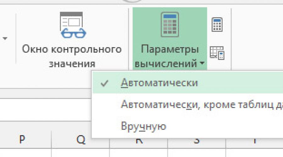
If you change the source data, but the formulas on the sheet do not want to be recalculated, you have disabled automatic recalculation of formulas.
To fix this, click on the ribbon: Formulas – Calculations – Calculation Options – Automatic. Now everything will be recalculated as usual.

Please remember that automatic recalculation may have been disabled on purpose. If you have a huge number of formulas on your worksheet, every change you make forces them to be recalculated. As a result, working with a document develops into a chronic state of waiting after each change. In this case, you need to convert the conversion to manual mode: Formulas – Calculations – Calculation Options – Manual. Now make all changes to the source data, the program will wait. When all changes have been made, press F9, all formulas will update the values. Or turn on automatic recalculation again.
If the cell is filled with a hash sign
Another classic situation when, as a result of calculations, you get not a result, but a cell filled with pound signs:

In fact, this is not an error, the program tells you that the result does not fit into the cell, it just needs to be adjusted to the required size.
The calculation result is in the wrong format
Sometimes it happens that after performing calculations, the result does not appear in the form you expect. For example, we added two numbers and got a date as a result. Why is this happening? It is likely that the data format in the cell was previously set to "date". Just change it to the one you need, and everything will be your way.
When external links are not available
If Excel formula returns incorrect result
If you have written a formula, and it returns an obviously incorrect result, let’s look at the logic of the formula. You could have made a simple mistake in the parentheses and the order of the operators. Study and check if everything is correct in yours. If correct, move on to the next step.
If you use functions, make sure you know. Each of them has its own syntax. Check whether you have set the parameters for the formula correctly by reading the help on it. Press F1 and in the Excel Help window, in the search, write your function, for example, “”. The program will display a list of available materials for this function. As a rule, they are enough to get a complete picture of how your function works. The authors of the help present the material in a very accessible way and provide examples of use.

Users often incorrectly specify cell references in formulas, which is why they get erroneous results. The first thing you need to do to test external formulas is to enable the display of formulas in cells. To do this, run on the ribbon Formulas – Formula Dependencies – Show Formulas. Now the cells will display formulas rather than calculation results. You can run your eyes over the sheet and check if the links are correct. To show the results again, run the same command again.
To make the process easier, you can turn on link arrows. You can easily determine which cells a formula refers to by clicking Formulas - Formula Dependencies - Influencing Cells. On the sheet, blue arrows will indicate which data you are referring to.

Similarly, you can see cells whose formulas refer to a given cell. To do this we do: Formulas – Formula Dependencies – Dependent Cells.
Please note that in complex tables, drawing arrows will take a lot of time and machine resources. To remove arrows, click Formulas – Formula Dependencies – Remove Arrows.
Typically, carefully checking formulas with the tools listed above will solve problems of erroneous results. We are looking for a problem until we win!
If a circular reference occurs in Excel
Sometimes after entering a formula, the program warns that a cyclic reference has been entered. The calculation stops. This means that the formula refers to a cell, which, in turn, refers to the cell in which you enter the formula. It turns out that there is a closed cycle of calculations, the program will have to calculate the result indefinitely. But this will not happen, you will be warned and given the opportunity to fix the problem.

Often, cells refer to each other indirectly, i.e. not directly, but through intermediate formulas.
To find such “incorrect” formulas, look on the ribbon: Formulas – Formula Dependencies – Error Checking – Cyclic Errors. This menu opens a list of cells with looped formulas. Click on any one to place the cursor in it and check the formula.
Naturally, circular references are eliminated by checking and correcting the calculation logic. However, in some cases, a circular reference will not be an error. That is, this system of formulas still needs to be calculated to a state close to equilibrium, when practically no changes occur. Some engineering problems require this. Luckily, Excel allows this. This approach is called “iterative calculations”. To turn them on, click File – Options – Formulas, and check the “Iterative calculations” checkbox. Install there:
- Limit iteration number– the maximum number of iterations (cycles) that will be carried out until a complete stop
- Relative error– the minimum change in target values during one iteration at which the recalculation will be stopped.
That is, the cyclic formula will be calculated until the relative error is reached, but not more than the specified maximum number of iterations.
Built-in Excel errors
Sometimes during calculations there are errors starting with the “#” sign. For example, “#N/A”, “#NUMBER!”, etc. these errors are me, read this post and try to understand the reason for your error. When this happens, you can easily fix everything.
If you cannot find an error in a rather complex formula, click on Exclamation point near the cell and in context menu select Show Calculation Steps.

A window will appear on the screen displaying at which point in the calculation the error occurs; it will be underlined in the formula. This the right way understand what exactly is wrong.

These are, perhaps, all the main ways to find and correct errors in Excel. We looked at the most common problems and how to fix them. But I’ll tell you what to do when errors need to be foreseen immediately in the calculations in a post about . Do not spare 5 minutes of time for this article; reading it carefully will save a lot of time in the future.
And I look forward to your questions and comments on this post!
Date: December 24, 2015 Category:Errors in Excel are an indispensable companion for everyone who... When an expression in a cell cannot be evaluated, the program displays an error message in the cell. It begins with a "#" followed by the name of the error. There is no need to be afraid of this if you are familiar with Excel functions and know how to follow the simplest logic of mathematical operations - you will easily find and correct the error.
If a cell is completely filled with pound signs (#), this is not an error at all. There is not enough space in the cell to display the result. Increase the cell size or decrease the font size so that the result can be displayed.
Types of errors
If an error does occur, decryption will help in correcting it:
| Error | Description |
| #DIV/0! | An error occurs when trying to divide by zero |
| #NAME? | The program cannot recognize the entered name. For example, you misspelled the function name, or did not enclose the text string in quotes |
| #N/A | Data not available. For example, I didn’t find any value |
| #EMPTY! | You requested the intersection of ranges that do not intersect |
| #NUMBER! | The problem is with one of the numeric values used in the formula. For example, you are trying to take the square root of a negative number. In classical mathematics this operation makes no sense |
| #LINK! | The formula contains a link that does not exist. For example, you deleted the cell it refers to |
| #VALUE! | The formula contains invalid components. Often this error occurs when the syntax of formulas is violated. |
When there is an error in a formula in a cell, a marker appears next to it. By clicking on it, you can read help about this error. You can also see the stages of calculation. Select this item, and the program will show a window where the location of the error will be underlined. This The best way determine where the error occurs.
In addition, you can do without correcting such errors, but simply . But it must be appropriate. Errors should only be worked around if they cannot be corrected. Otherwise, the calculation results may be distorted.
 Tracing an error through calculation steps
 Circular links in Excel
Another type of error is a circular reference. It occurs when you reference a cell whose value depends on the one in which you write the formula. For example, in a cage A1 the formula =A2+1 is written, and in A2 write =A1 , a cyclic reference will appear that will be recalculated endlessly. In this case, the program warns about the appearance of a cyclic reference and stops the calculation of “cyclic formulas”. A double-headed arrow appears on the left side of the cells. You will have to correct the error that occurred and repeat the calculation.

Sometimes complex “looping” occurs when a cyclic link is formed with several intermediate formulas.
To track down such errors, run Formulas – Formula Dependencies – Error Checking – Circular References. In the drop-down list, the program displays the addresses of the cells that create an endless loop. All that remains is to correct the formulas in these cells.
 Tracking Circular Links
 In Excel, you can try to calculate the result of looping formulas. To do this, check the box File – Options – Formulas – Enable Iterative Calculations. In the same block, you can set the maximum number of iterations (calculations) to find the balance and the permissible error. In most cases this is not necessary, so I recommend not checking this box. However, when you know that the looping formulas are correct and their calculation will lead to a stable result - why not do it?
That's all about the types of errors in Excel. This short article has given you enough information to deal with the most common errors in Excel by analyzing the return value. But read the extended list of errors in! I’m ready to answer your questions - write in the comments.
In the next article I will tell you. Needless to say that Excel functions are “our everything”?
I think no. Therefore, go ahead and read, this will be the first step into the world complex formulas with the right results!
Making even a small change at work Excel sheet may lead to errors in other cells. For example, you might accidentally enter a value in a cell that previously contained a formula. This simple mistake can have a significant impact on other formulas, and you may not be able to detect it until you make some changes to the worksheet.
Errors in formulas fall into several categories:
Syntax errors: Occurs when the formula syntax is incorrect. For example, a formula has incorrect parentheses, or a function has the wrong number of arguments.
Logical errors: In this case, the formula does not return an error, but has a logical flaw, which causes the calculation to be incorrect.
Invalid link errors: The formula logic is correct, but the formula uses an incorrect cell reference. As a simple example, the range of data to be summed in the SUM formula may not contain all the items you want to sum.
Semantic errors: For example, the name of the function is misspelled, in which case Excel will return the error #NAME?
Errors in array formulas: When you enter an array formula, you must press Ctrl + Sift + Enter when you finish typing. If you don't do this, Excel won't realize it's an array formula and will return an error or incorrect result.
Errors in incomplete calculations: In this case, the formulas are not fully calculated. To make sure that all formulas are recalculated, type Ctrl + Alt + Shift + F9.
The easiest way is to find and correct syntax errors. More often than not, you know when a formula contains a syntax error. For example, Excel will not allow you to enter a formula with inconsistent parentheses. Other syntax error situations result in the following errors being displayed in the worksheet cell.
Error #DIV/0!
If you create a formula that divides by zero, Excel will return the error #DIV/0!
Since Excel treats an empty cell as zero, dividing by an empty cell will also return an error. This problem often occurs when creating a formula for data that has not yet been entered. The formula in cell D4 has been stretched across the entire range (=C4/B4).

This formula returns the ratio of the values of columns C to B. Since not all data for days was entered, the formula returned the error #DIV/0!
To avoid the error, you can use , to check whether the cells of column B are empty or not:
IF(B4=0;"";C4/B4)
This formula will return empty value, if cell B4 is empty or contains 0, otherwise you will see the counted value.
Another approach is to use the ISERROR function, which checks for an error. The following formula will return an empty string if the expression C4/B4 returns an error:
IFERROR(C4/B4;"")
Error #N/A
The #N/A error occurs when the cell referenced by the formula contains #N/A.
Typically, the #N/A error is returned as a result of running . In the case where no match was found.
To catch the error and display an empty cell, use the =ESND() function.
ESND(VLOOKUP(A1,B1:D30,3,0);"")
Please note that the ESND function is new feature in Excel 2013. For compatibility with previous versions use an analogue of this function:
IF(END(VLOOKUP(A1,B1:D30,3,0));"";VLOOKUP(A1,B1:D30,3,0))
Error #NAME?
Excel may return the error #NAME? in the following cases:
- Formula contains an undefined named range
- The formula contains text that Excel interprets as an undefined named range. For example, a misspelled function name will return the error #NAME?
- The formula contains text not enclosed in quotation marks
- The formula contains a reference to a range that does not have a colon between the cell addresses
- The formula uses a worksheet function that was defined by an add-in, but the add-in was not installed
Error #EMPTY!
Error #EMPTY! occurs when a formula tries to use the intersection of two ranges that do not actually intersect. The intersection operator in Excel is space. The following formula will return #EMPTY! because the ranges do not overlap.

Error #NUMBER!
Error #NUMBER! will be refunded in the following cases:
- A non-numeric value was entered into a formula's numeric argument (for example, $1,000 instead of 1000)
- An invalid argument was entered into the formula (for example, =ROOT(-12))
- A function that uses iteration cannot calculate the result. Examples of functions that use iteration: VSD(), BET()
- The formula returns a value that is too large or too small. Excel supports values between -1E-307 and 1E-307.
Error #LINK!
- You deleted a column or row that was referenced by a formula cell. For example, the following formula will return an error if the first row or columns A or B were deleted:
- You deleted the worksheet that was referenced by a formula cell. For example, the following formula will return an error if Sheet1 was removed:
- You copied the formula to a location where the relative reference becomes invalid. For example, if you copy a formula from cell A2 to cell A1, the formula will return a #REF! error because it is trying to reference a cell that does not exist.
- You cut the cell and then paste it into the cell referenced by the formula. In this case, the error #LINK! will be returned.
Error #VALUE!
Error #VALUE! is the most common error and occurs in the following situations:
- The function argument has the wrong data type or the formula is trying to perform an operation using the wrong data. For example, when trying to add a numeric value to a text value, the formula will return an error
- Function argument is a range when it should be a single value
- Custom sheet functions are not calculated. To force a recalculation, press Ctrl + Alt + F9
- A custom worksheet function attempts to perform an operation that is not valid. For example, a custom function cannot change the Excel environment or make changes to other cells
- You forgot to press Ctrl + Shift + Enter when entering an array formula