Calculations in Excel
A formula is a mathematical expression that is created to calculate a result and that may depend on the contents of other cells. A formula in a cell can contain data, references to other cells, and an indication of the action to be taken.
Using cell references allows formula results to be recalculated when the contents of cells included in formulas change.
In Excel, formulas start with an = sign. Parentheses () can be used to specify the order of mathematical operations.
Excel supports the following operators:
- Arithmetic operations:
- addition (+);
- multiplication (*);
- finding the percentage (%);
- subtraction (-);
- division (/);
- exponent (^).
- Comparison operators:
- = equal;
- < меньше;
- > more;
- <= меньше или равно;
- >= greater than or equal;
- <>not equal.
- Telecom operators:
- : range;
- ; Union;
- & text join operator.
Table 22. Formula examples
Exercise
Insert formula -25-A1+AZ
Pre-enter any numbers in cells A1 and A3.
- Select the desired cell, for example B1.
- Start entering a formula with the = sign.
- Enter the number 25 followed by the operator (sign -).
- Enter a reference to the first operand, for example by clicking on the desired cell A1.
- Enter the following operator (+ sign).
- Click in the cell that is the second operand in the formula.
- Finish entering the formula by pressing the key Enter. In cell B1, get the result.
Autosummation
Button Autosum (AutoSum)- ∑ can be used to automatically create a formula that sums the area of neighboring cells that are directly left in this line and directly higher in this column.
- Select the cell where you want to place the result of the summation.
- Click the AutoSum - ∑ button or press the keyboard shortcut Alt+=. Excel will decide which area to include in the summation range and highlight it with a dotted moving box called a border.
- Click Enter to accept the area that Excel has selected, or use the mouse to select a new area and then press Enter.
The AutoSum function automatically transforms when cells are added and removed within the area.
Exercise
Creating a table and calculating by formulas
- Enter numeric data in the cells, as shown in the table. 23.
| A | IN | WITH | D | B | F | |
| 1 | ||||||
| 2 | Magnolia | Lily | Violet | Total | ||
| 3 | Higher | 25 | 20 | 9 | ||
| 4 | Average spec. | 28 | 23 | 21 | ||
| 5 | vocational school | 27 | 58 | 20 | ||
| V | Other | 8 | 10 | 9 | ||
| 7 | Total | |||||
| 8 | Without higher |
Table 23. Initial data table
- Select cell B7, in which the vertical sum will be calculated.
- Click the AutoSum - ∑ button or click Alt+=.
- Repeat steps 2 and 3 for cells C7 and D7.
Calculate the number of employees without higher education (using the B7-B3 formula).
- Select cell B8 and type the (=) sign.
- Click in cell B7, which is the first operand in the formula.
- Enter the (-) sign on the keyboard and click in the OT cell, which is the second operand in the formula (the formula will be entered).
- Click Enter(in cell B8 the result will be calculated).
- Repeat steps 5-8 to calculate the corresponding formulas in cells C8 and 08.
- Save the file with the name Education_Employees.x1s.
Table 24Calculation result
| A | B | WITH | D | E | F | |
| 1 | Distribution of employees by education | |||||
| 2 | Magnolia | Lily | Violet | Total | ||
| 3 | Higher | 25 | 20 | 9 | ||
| 4 | Average spec. | 28 | 23 | 21 | ||
| 5 | vocational school | 27 | 58 | 20 | ||
| 6 | Other | 8 | 10 | 9 | ||
| 7 | Total | 88 | 111 | 59 | ||
| 8 | Without higher | 63 | 91 | 50 | ||
Duplicate formulas using the fill handle
A cell area (cell) can be replicated by using fill marker. As shown in the previous section, the fill handle is the breakpoint in the lower right corner of the selected cell.
Often it is necessary to multiply not only data, but also formulas containing address links. The process of replicating formulas using a fill handle allows you to colorize a formula while changing the address references in the formula.
- Select the cell containing the formula to replicate.
- Drag fill marker in the right direction. The formula will be duplicated in all cells.
Typically, this process is used when copying formulas within rows or columns containing data of the same type. When replicating formulas using a fill marker, the so-called relative cell addresses in the formula change (relative and absolute references will be described in detail later).
Exercise
Replication of formulas
1.Open the file Education_Employees.x1s.
- Enter in cell E3 the formula for autosumming cells = SUM (OT: 03).
- Drag and drop the fill handle to copy the formula into cells E4:E8.
- See how the relative cell addresses change in the resulting formulas (Table 25) and save the file.
| A | IN | WITH | D | E | F | |
| 1 | Distribution of employees by education | |||||
| 2 | Magnolia | Lily | Violet | Total | ||
| 3 | Higher | 25 | 20 | 9 | =SUM(VZ:03) | |
| 4 | Average spec. | 28 | 23 | 21 | =SUM(B4:04) | |
| 5 | vocational school | 27 | 58 | 20 | =SUM(B5:05) | |
| 6 | Other | 8 | 10 | 9 | =SUM(B6:06) | |
| 7 | Total | 88 | 111 | 58 | =SUM(B7:07) | |
| 8 | Without higher | 63 | 91 | 49 | =SUM(B8:08) | |
Table 25. Changing cell addresses when replicating formulas
Relative and absolute links
Formulas that implement calculations in tables use so-called links to address cells. Cell reference can be relative or absolute.
The use of relative references is similar to indicating the direction of travel along the street - "go three blocks north, then two blocks west." Following these instructions from different starting places will lead to different destinations.
For example, a formula that sums the numbers in a column or row is then often copied to other row or column numbers. These formulas use relative references (see the previous example in Table 25).
An absolute cell reference. Go cell area will always refer to the same row and column address. When compared with the directions of the streets, it will be something like this: "Go to the intersection of the Arbat and the Boulevard Ring." Regardless of the starting point, this will lead to the same place. If the formula requires that the cell address remain unchanged when copied, then an absolute reference (record format $A$1) must be used. For example, when a formula calculates fractions of a total, the reference to the cell containing the total must not change when copied.
A dollar sign ($) will appear before both a column reference and a row reference (e.g. $C$2), Successive pressing F4 will add or remove a sign before the column or row number in the reference (C$2 or $C2 - the so-called mixed links).
- Create a table similar to the one below.
Table 26. Payroll
- In the SZ cell, enter the formula for calculating Ivanov's salary \u003d V1 * VZ.
When replicating the formula of this example with relative references in cell C4, an error message (#VALUE!) appears, since the relative address of cell B1 will change, and the formula =B2*B4 will be copied to cell C4;
- Set the absolute reference to cell B1 by placing the cursor in the formula bar on B1 and pressing the F4 key. The formula in cell C3 will look like =$B$1*B3.
- Copy the formula into cells C4 and C5.
- Save the file (Table 27) under the name Salary.xls.
Table 27. Payroll results
Names in formulas
Names in formulas are easier to remember than cell addresses, so you can use named scopes (single or multiple cells) instead of absolute references. The following rules must be observed when creating names:
- names can be up to 255 characters long;
- names must begin with a letter and may contain any character except a space;
- names should not look like links, such as OT, C4;
- names should not use Excel functions such as SUM IF and so on.
On the menu Insert, Name There are two different commands for creating named areas: Create and Assign.
Team Create allows you to set (enter) the required name ( only one), Assign command uses the labels placed on the worksheet as area names (it is allowed to create several names at once).
Making a name
- Select cell B1 (Table 26).
- Select from the menu Insert, Name (Insert, Name) command Assign (Define).
- Enter your name Hourly rate and click OK.
- Select cell B1 and make sure the name field says hourly rate.
Creating multiple names
- Select cells ВЗ:С5 (Table 27).
- Select from the menu Insert, Name (Insert, Name) command Create (Create), a dialog box will appear. Create names(Fig. 88).
- Make sure the radio button in the column on the left is checked and click OK.
- Highlight the cells OT:NW and make sure the name field says Ivanov.
Rice. Figure 88. Create Names Dialog Box
You can insert a name into a formula instead of an absolute reference.
- In the formula bar, position the cursor where the name will be added.
- Select from the menu Insert, Name (Insert, Name) command Paste (Paste), The Insert Names dialog box appears.
- Select the desired name from the list and click OK.
Errors in formulas
If an error is made when entering formulas or data, an error message appears in the resulting cell. The first character of all error values is #. Error values depend on the type of error made.
Excel can recognize far from all errors, but those that are found must be able to correct.
Error # # # # appears when the entered number does not fit in the cell. In this case, increase the column width.
Error #DIV/0! appears when an attempt is made to divide by zero in a formula. This most often happens when the divisor is a cell reference that contains a zero or blank value.
Error #N/A! is an abbreviation for "undefined data". This error indicates the use of an empty cell reference in the formula.
Error #NAME? appears when a name used in a formula has been removed or was not previously defined. To correct, define or correct the data area name, function name, etc.
Error #BLANK! appears when the intersection of two regions is specified, which do not actually have common cells. Most often, the error indicates that an error was made when entering cell range references.
Error #NUMBER! appears when an invalid format or argument value is used in a function with a numeric argument.
Error #VALUE! appears when an invalid argument or operand type is used in a formula. For example, text is entered instead of a numeric or boolean value for an operator or function.
In addition to the errors listed above, when entering formulas, a circular reference may appear.
A circular reference occurs when a formula directly or indirectly includes references to its own cell. A circular reference can cause distortion in worksheet calculations and is therefore considered a bug in most applications. When entering a circular reference, a warning message appears (Fig. 89).

To correct the error, delete the cell that caused the circular reference, edit or re-enter the formula.
Functions in Excel
More complex calculations in Excel tables are carried out using special functions (Fig. 90). The list of function categories is available when you select the command Function in the Insert menu (Insert, Function).
Financial functions perform such calculations as calculating the amount of payment on a loan, the amount of payment of profit on investments, etc.
The Date and Time functions allow you to work with date and time values in formulas. For example, you can use the current date in a formula by using the function TODAY.
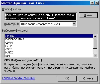
Rice. 90. Function Wizard
Math functions perform simple and complex mathematical calculations, such as calculating the sum of a range of cells, the absolute value of a number, rounding numbers, etc.
Statistical functions allow you to perform statistical analysis of the data. For example, you can determine the mean and variance of a sample, and much more.
Database Functions can be used to perform calculations and to select records by condition.
Text functions provide the user with the ability to process text. For example, you can concatenate multiple strings using the function CONNECT.
Boolean functions are designed to test one or more conditions. For example, the IF function allows you to determine whether the specified condition is true, and returns one value if the condition is true, and another value if it is false.
Functions Checking properties and values are intended to define the data stored in the cell. These functions check the values in the cell according to the condition and return the values depending on the result. TRUE or FALSE.
For table calculations using built-in functions, we recommend using the Function Wizard. The Function Wizard dialog box is available when you select the command Function in the Insert menu or pressing a button , on the standard toolbar. During the dialogue with the wizard, it is required to set the arguments of the selected function; for this, it is necessary to fill in the fields in the dialog box with the corresponding values or addresses of the table cells.
Exercise
Calculation of the average value for each line in the file Education.xls.
- Highlight cell F3 and click on the Function Wizard button.
- In the first dialog box of the Function Wizard, from the Statistical category, select a function AVERAGE, click on the button Further.
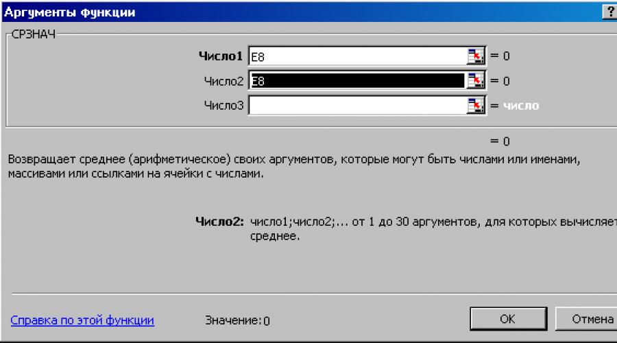
- Arguments must be given in the second dialog box of the function wizard. The input cursor is in the input field of the first argument. In this field as an argument number! enter the address of the range B3:D3 (Fig. 91).
- Click OK.
- Copy the resulting formula into cells F4:F6 and save the file (Table 28).
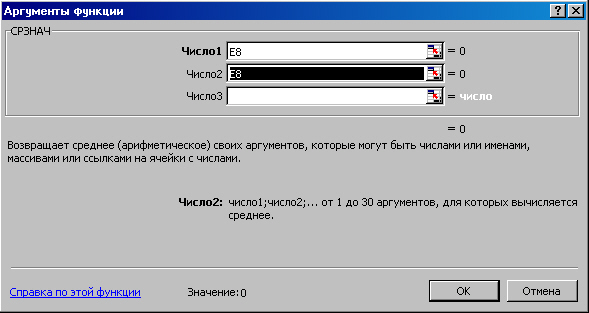
Rice. 91 Entering an Argument in the Function Wizard
Table 28. Table of calculation results using the function wizard
| A | IN | WITH | D | E | F | |
| 1 | Distribution of employees by education | |||||
| 2 | Magnolia | Lily | Violet | Total | Average | |
| 3 | Higher | 25 | 20 | 9 | 54 | 18 |
| 4 | Average spec. | 28 | 23 | 21 | 72 | 24 |
| 8 | vocational school | 27 | 58 | 20 | 105 | 35 |
| V | Other | 8 | 10 | 9 | 27 | 9 |
| 7 | Total | 88 | 111 | 59 | 258 | 129 |
To enter a range of cells in the function wizard window, you can circle this range on the worksheet of the table (in the example B3:D3). If the Function Wizard window covers the desired cells, you can move the dialog box. After selecting a range of cells (B3:D3), a running dotted frame will appear around it, and the address of the selected range of cells will automatically appear in the argument field.