How to calculate the sum in a table in Excel (Excel): general formulas automatically

How to calculate sum in excel spreadsheet?
Today we have a topic for novice users of Microsoft Office Excel (Excel), namely: how to correctly calculate the sum of digits?
Excel (Excel) is one of the programs of the Microsoft Office package designed to work with data tables. Compatible with Windows and MacOS operating systems and OpenOffice software product.

Since Excel (Excel) is ready-made tables with cells for placing data, it can perform arithmetic operations in them with groups of data vertically and horizontally, as well as with individual cells, or individual groups of cells.

Now separately we will focus on how to calculate the amount.
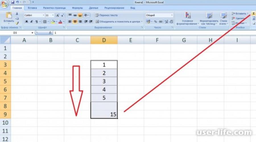
1. Select the desired range of cells with numbers vertically, continuing the selection two empty cells below and click the "Calculate amount" icon in the program menu.

2. Select the desired range of cells with numbers horizontally, continuing the selection two empty cells below and click the "Calculate amount" icon in the program menu.

3. You can add individual cells located in different rows and columns. To do this, in Excel (Excel), you must select an empty cell and write the sum formula. Equals (=), select cell 1+ cell 5+ cell N and press Enter.

By the way, this way you can not only get the amount, but also multiply, divide, subtract and apply more complex formulas.

So, first you need to left-click on any cell and write the following in it: “=500+700” (without quotes). After pressing the "Enter" button, the result will be 1200. In this simple way, you can add 2 numbers. Using the same function, you can perform other operations - multiplication, division, etc. In this case, the formula will look like this: “number, sign, number, Enter”. This was a very simple example of adding 2 numbers, but, as a rule, it is used quite rarely in practice.

Name;
quantity;
price;
sum.
In total, the table has 5 items and 4 columns (all filled in, except for the amount). The task is to find the sum for each product.

For example, the first name is a pen: the quantity is 100 pieces, the price is 20 rubles. To find the sum, you can use the simple formula that has already been discussed above, i.e. write like this: "=100×20". Of course, you can use this option, but it will not be entirely practical. Let's say the price of a pen has changed, and now it costs 25 rubles. And what to do then - rewrite the formula? And if the table of product names is not 5, but 100 or even 1000? In such situations, Excel can get the sum of numbers in other ways, incl. recalculating the formula if one of the cells changes.

To calculate the amount in a practical way, you need a different formula. So, first you need to put an "equal" sign in the corresponding cell of the "Amount" column. Next, you need to left-click on the number of pens (in this case it will be the number "100"), put the multiplication sign, and then left-click again on the price of the pen - 20 rubles. After that, you can press "Enter". It seems that nothing has changed, since the result remained the same - 2000 rubles.

But there are two nuances here. The first is the formula itself. If you click on a cell, you can see that not numbers are written there, but something like “=B2*C2”. The program did not write numbers to the formula, but the name of the cells in which these numbers are located. And the second nuance is that now when you change any number in these cells (“Quantity” or “Price”), the formula will be automatically recalculated.
If you try to change the price of a pen by 25 rubles, then another result will immediately be displayed in the corresponding “Amount” cell - 2500 rubles. That is, when using such a function, it will not be necessary to independently recalculate each number if some information has changed. You just need to change the original data (if necessary), and Excel will automatically recalculate everything.

After that, the user will have to calculate the amount and the remaining 4 items. Most likely, the calculation will be made in a way familiar to him: an equal sign, a click on the “Quantity” cell, a multiplication sign, another click on the “Price” cell and “Enter”. But in Microsoft Excel, there is one very interesting function for this, which allows you to save time by simply copying the formula into other fields.

So, first you need to select the cell in which the total amount of pens has already been calculated. The selected cell will be highlighted with thick lines, and there will be a small black square in the lower right corner. If you correctly hover over this box with the mouse, then the appearance of the cursor will change: instead of a white “plus sign”, there will be a black “plus sign”. At the moment when the cursor looks like a black plus sign, you need to left-click on this lower right square and drag it down until the desired moment (in this case, 4 lines down).

This manipulation allows you to "pull" the formula down and copy it into 4 more cells. Excel will instantly show you all the results. If you click on any of these cells, you can see that the program independently wrote the necessary formulas for each cell and did it absolutely correctly. This manipulation will be useful if there are a lot of items in the table. But there are some limitations here.

First, the formula can only be "pulled" down/up or sideways (i.e. vertically or horizontally). Secondly, the formula must be the same. Therefore, if the sum is calculated in one cell, and the numbers are multiplied in the next (under it), then such manipulation will not help, in this case it will copy only the addition of numbers (if the first cell was copied).

How to calculate the amount using the "AutoSum" function?
Another way to calculate the sum of numbers is using the AutoSum function. This feature is usually found in the toolbar (just below the menu bar). AutoSum looks like the Greek letter E. So, for example, there is a column of numbers, and you need to find their sum. To do this, select the cell under this column and click the "AutoSum" icon. Excel will automatically select all the cells vertically and write the formula, and the user will only have to press "Enter" to get the result.