How to add numbers in cells in EXCEL according to a certain condition

Many people working with EXCEL spreadsheets at some point are faced with the question "how to add numbers in cells in EXCEL according to a certain condition." On one of the sunny days, I also encountered this question, but I did not find the answer to this question on the Internet, but I was persistent and decided to study the help of the program, which prompted me to think, and then by trial and error I made a formula, and as it turned out, the formula is elementary.

It all started with the fact that I decided to take into account my monthly expenses and for this I created a table that I attached to this article, because it can be useful to you too.

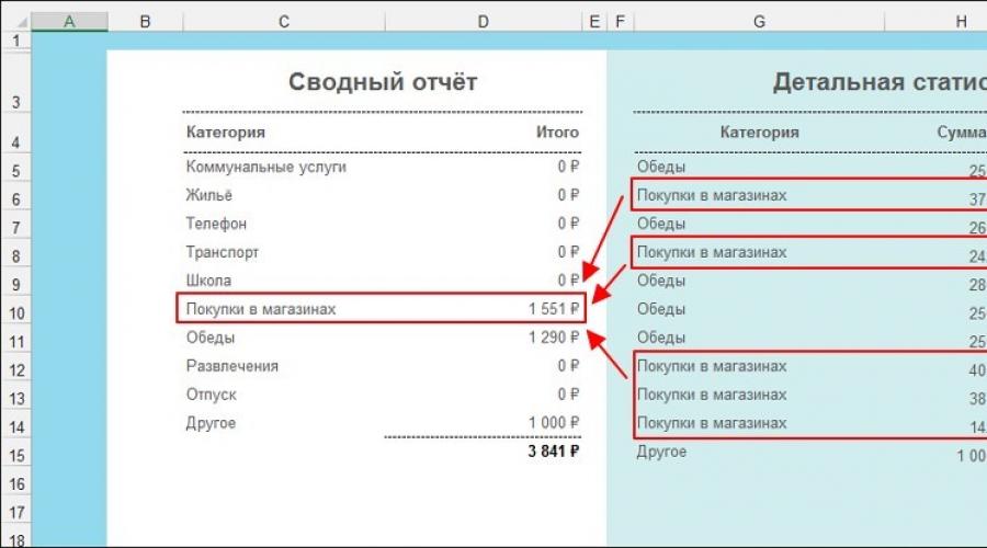
Now I will try to describe in detail the principle of creating a formula. I have detailed statistics and a summary report in the report. In the detailed statistics, I enter my daily expenses, and in the summary report, the amount of expenses for certain categories and the total amount of expenses are considered.

For example, let's take the category of expenses "Shopping in stores". We need EXCEL to find all the costs for this category in detailed statistics, summarize the costs for this category and write the resulting amount into a cell D10.

First, write down the finished formula, which we insert into the cell D10 and then we'll get into the details. The finished formula looks like this (only for our article):

=SUMIF ($G$5:$G$300 ;(" Shopping in stores");$H$5:$H$300 )

Different conditions are highlighted in color to make it clearer. Let's take it in order. In the process of description, look at the picture above to make it clearer. When taking a picture, the letters of the columns and the numbers of the rows were specially captured. So let's get started.

• SUMIF- with this condition, we say that the sum of the values ​​​​of certain cells should be written to the cell if they meet certain conditions;
• $G$5:$G$300- here we tell EXCEL in which column we need to look for a condition for the selection. In our case, the search occurs in the column G starting from line 5 and ending with the line 300 ;
• (« Shopping in stores») - here we indicate the desired condition, and according to this condition, the values ​​​​of the cells that we indicate below will be summed up ...;
• $H$5:$H$300- here we specify the column from which the numbers will be taken for summation. In our case, the values ​​are taken in the column H starting from line 5 and ending with the line 300.

Summing up, we can say that EXCEL sums only those values ​​from the range H5:H300, for which the corresponding values ​​from the range G5:G300 are equal to "Purchases in stores" and writes the result in a cell D10.

In an appropriate way, you can in excel add numbers in cells according to any condition.

Sign $ in the formula is used so that when copying the formula from cell D10 to other cells, there is no shift. Consider an example of an unsigned formula $ . For example, in a cell D10 we have the formula:

=SUMIF(G5:G300,("Store shopping");H5:H300)

Next, we want to display the sum of the meals in the cell D11. In order for us not to rewrite the formula, we can copy the cell D10 and paste into cell D11. This will insert the formula into D11, but here we can notice that the formula has changed the values ​​by replacing 5 with 6 and 300 with 301:

=SUMIF(G6:G301,("Shopping");H6:H301)

A shift has occurred. If we copy the formula to D12, then we will already see an offset of 2 and so on. To avoid this, we write the formula with a sign $ . Such features of EXCEL.

Table "Accounting for monthly expenses" -