How to make a complex drop down list in excel?
If you are filling out a table in Excel, and the data in a column can sometimes be repeated, for example, the name of a product, or the name of an employee, then in order not to enter the required parameter each time, it is easier and easier to create a drop-down list once and select a value from it.
In the article, we will look at how to make drop-down lists of various types in an Excel spreadsheet.
Create a simple drop down list
To do this, in cells A1: A7 we enter the data that will be displayed in the list. Now select the cell in which we will create a drop-down list - B2.
Go to the "Data" tab and click on the "Data Validation" button.
On the "Options" tab, in the "Data type" field, select "List". You can enter values in the Source field in various ways:
1 - enter the values for the list manually, separated by a semicolon;

2 - specify the range of cells in which the data for the drop-down list is entered;

3 - select the cells with names, right-click on them and select "Assign a name" from the menu.


Select cell B2 and put "=" in the "Source" field, then write the created name.

Thus, we have created a simple drop down list in Excel.
If you have a header for a column, and you need to fill in each row with values, then select not one cell, but a range of cells - B2:B9. Then it will be possible to select the desired value in each cell from the drop-down list.

Adding Values to the Dropdown List - Dynamic List
In this case, we will add values to the desired range, and they will be automatically added to the drop-down list.
Select the range of cells - D1:D8, then on the "Home" tab, click "Format as Table" and select any style.

We confirm the location of the data and put a tick in the field "Table with headers".
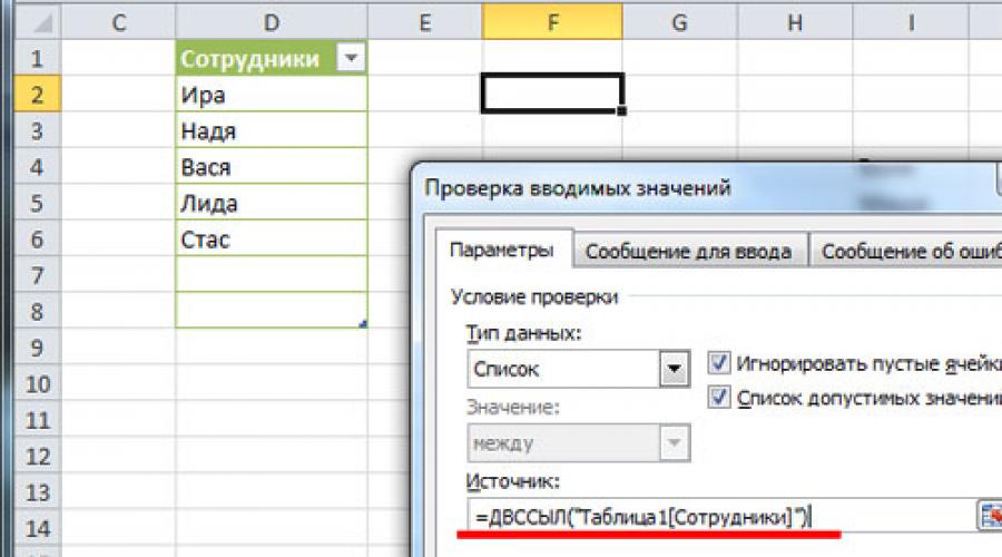
At the top we write the title of the table - "Employees", and fill it with data.
Select the cell that will contain the drop-down list and click on the "Data Validation" button. In the next window, in the "Source" field, write the following: =INDIRECT("Table1"). I have one table on a sheet, so I write “Table1”, if there is a second one - “Table2”, and so on.

Now let's add a new employee name to our list: Ira. It appeared in the dropdown list. If we remove any name from the table, it will also be removed from the list.

Dropdown list with values from another sheet
If the table with drop-down lists is on one sheet, and the data for these lists is on another, then this function will help us a lot.
On Sheet 2, select one cell or range of cells, then click on the "Data Validation" button.

Go to Sheet 1, put the cursor in the "Source" field and select the desired range of cells.

Now you can add names on Sheet 1, they will be added to the drop-down lists on Sheet 2.
Creating dependent dropdown lists
Let's say we have three ranges: first names, last names, and middle names of employees. For each, you need to assign a name. We select the cells of this range, it can also be empty - over time, it will be possible to add data to them that will appear in the drop-down list. We click on them with the right mouse button and select "Assign a name" from the list.

The first is called "Name", the second - "Surname", the third - "Father".

Let's make another range in which the assigned names will be written. Let's call it "Employees".

We make the first drop-down list, which will consist of the names of the ranges. Select cell E1 and on the Data tab, select Data Validation.
In the "Data type" field, select "List", in the source field - either enter "=Employees", or select a range of cells that has been given a name.
The first dropdown list has been created. Now in cell F2 we will create a second list, which should depend on the first one. If we select “First Name” in the first one, the list of surnames will be displayed in the second one, if we select “Last Name” - a list of surnames.
Select the cell and click on the Data Validation button. In the "Data type" field, select "List", in the source field, enter the following: =INDIRECT($E$1). Here E1 is the cell with the first drop down list.
By this principle, you can make dependent drop-down lists.
If in the future, you will need to enter the values in the range to which the name is given, for example, "Last name". Go to the "Formulas" tab and click "Name Manager". Now, in the name of the range, select "Last Name", and at the bottom, instead of the last cell C3, write C10. Click the checkmark. After that, the range will increase, and it will be possible to add data to it, which will automatically appear in the drop-down list.
Now you know how to make a drop down list in Excel.
How to create a drop-down list consisting of several cells at once (let's say that the name is with a cost)
Thanks, all worked well.
The drop-down list with values from another sheet does not work, since the window when the data check is open does not allow working with other windows, especially with another sheet!
Dependent dropdown allows you to do a trick that is often praised by users of Excel templates. A trick that makes the job easier and faster. A trick that will make your forms comfortable and pleasant.
An example of creating a dependent dropdown list in an Excel cell
An example of using a dependent drop-down list to create a convenient form for filling out documents with which sellers ordered goods. From the entire assortment, they had to choose those products that they were going to sell.
Each seller first identified a product group, and then a specific product from this group. The form must include the full name of the group and a specific item index. Since typing this by hand would be too time consuming (and annoying) I came up with a very quick and easy solution - 2 dependent dropdowns.
The first was a list of all product categories, the second was a list of all products in the selected category. Therefore, I created a dropdown list dependent on the selection made in the previous list (here you will find material on how to create two dependent dropdown lists).
The user of the home budget template wants to get the same result, where the category and subcategory of expenses are needed. An example of data is in the figure below:
So, for example, if we select the category Entertainment, then the list of subcategories should be: Cinema, Theater, Pool. A very quick solution if you want to analyze more detailed information in your home budget.
List Categories and Subcategories in Excel Dependent Dropdown
I confess that in my proposed version of the home budget, I am limited to only a category, since for me such a division of expenses is quite enough (the name of expenses / incomes is considered as a subcategory). However, if you need to subcategorize them, then the method I describe below is ideal. Feel free to use!
And the end result looks like this:
Dependent dropdown list of subcategories
In order to achieve this, we need to make a slightly different data table than if we were creating a single drop-down list. The table should look like this (range G2:H15):
Working source Excel spreadsheet
In this table, you must enter a category and next to it its subcategories. The category name must be repeated as many times as there are subcategories. It is very important that the data is sorted by the Category column. This will be extremely important when we write the formula later.
One could also use the tables from the first image. Of course, the formulas would be different. Once even I found such a solution on the net, but I did not like it, because there was a fixed length of the list: which means that sometimes the list contained empty fields, and sometimes it did not display all the elements. Of course, I can avoid this limitation, but I confess that I like my solution better, so I did not return to that solution.
OK then. Now, one by one, I will describe the steps for creating a dependent dropdown list.
1. Cell range names
This is an optional step, without it we should be able to handle this without any problems. However, I like to use names because they make it much easier to both write and read the formula.
Let's name the two ranges. List of all categories and working list of categories. These will be the ranges A3:A5 (the list of categories in the green table in the first image) and G3:G15 (the list of duplicate categories in the purple worksheet).
To name a list of categories:
- Select range A3:A5.
- In the name field (the field to the left of the formula bar), enter the name "Category".
- Confirm with the Enter key.
Do the same for the category worklist range G3:G15, which you can call WorkList. We will use this range in the formula.
2. Create a dropdown list for a category
It will be simple:
- Select the cell where you want to place the list. In my case it is A12.
- From the DATA menu, select the Data Validation tool. The Validate Input Values window appears.
- Select "List" as the data type.
- For the source, enter: =Category (picture below).
- Confirm with OK.
The result is the following:
Dropdown list for category.
3. Create a dependent dropdown list for a subcategory
Now it will be fun. We know how to create lists - we just did it for a category. Only one question: "How do I tell Excel to select only those values that are for a particular category?" As you can probably guess, I will be using a worksheet here and, of course, formulas.
Let's start with what we already know, which is to create a drop-down list in cell B12. So select that cell and click Data/Data Validation and set the data type to List.
In the list source, enter the following formula:
View of the "Check input values" window:
Validation of input values for a subcategory in a dependent dropdown list
As you can see, the whole dependent list trick is to use the OFFSET function. Well, almost all. The MATCH and COUNTIF functions help her. The OFFSET function allows you to dynamically define ranges. First, we define the cell from which the range shift should start, and in subsequent arguments we define its size.
In our example, the range will move across the Subcategory column in the worksheet (G2:H15). We will start moving from cell H2, which is also the first argument of our function. In the formula, cell H2 is written as an absolute reference, because I assume that we will use the drop-down list in many cells.
Because the worksheet is sorted by Category, the range that should be the source for the drop-down list will begin where the selected category first occurs. For example, for the Food category, we want to display the range H6:H11, for the Transport category, the range H12:H15, and so on. Note that we are moving along column H all the time, and the only thing that changes is the beginning of the range and its height ( i.e. the number of elements in the list).
The beginning of the range will be moved relative to cell H2 by as many cells down (in number) as the position number of the first occurring category in the Category column. It will be easier to understand with an example: the range for the Food category is moved 4 cells down relative to cell H2 (starts from 4 cells from H2). In the 4th cell of the Subcategory column (not including the heading, as it is a range named WorkList), there is the word Food (its first occurrence). We use this fact to actually determine the beginning of the range. The MATCH function will serve us for this (introduced as the second argument of the OFFSET function):
The height of the range is determined by the COUNTIF function. She counts all occurrences in the category, that is, the word Nutrition. How many times this word occurs, how many positions will be in our range. The number of positions in a range is its height. Here is the function:
Of course, both functions are already included in the OFFSET function described above. Also note that in both MATCH and COUNTIF, there is a reference to a range called WorkList. As I mentioned earlier, you don't have to use range names, you can just type $H3: $H15. However, using range names in a formula makes it simpler and easier to read.
That's all:
Download Dependent Dropdown List Example in Excel
One formula, well, not so simple, but it makes work easier and protects against data entry errors!