How to work with dropdown list in Excel
Work in Excel with tables and data in them is built in such a way that the user can comfortably process and analyze them. To do this, various tools are built into the program. Their use requires the user to have some knowledge, but with them, Excel turns into a powerful analysis tool. The Office developer tries to simplify most of his programs so that anyone can fully use them.
Spreadsheet can be turned into a data analysis tool
Sometimes it becomes necessary for the author of a document to restrict input. For example, in a certain cell, only data from a predefined set should be entered. Excel makes this possible.
One of the most common reasons for creating a pop-up list is to use data from a cell in an Excel formula. It is easier to provide a finite number of options, so it is advisable to give a choice of several values so that the user can choose from a ready set. In addition, there may be another reason: a predefined document style. For example, for reports or other official documents. The same department name can be written in different ways. If this document is later processed by a machine, it will be more correct to use a uniform filling style, and not set it to the task of recognition, for example, by keywords. This may introduce an element of inaccuracy into its work.
The technical side of the issue
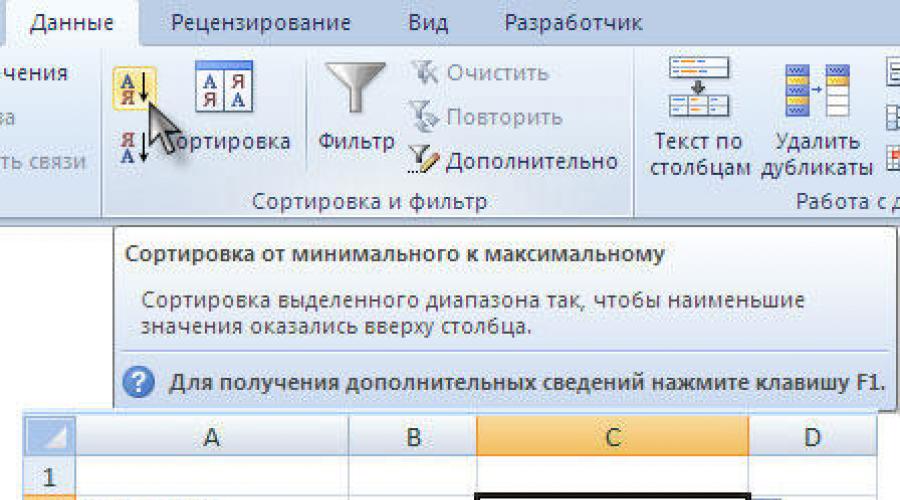
Before you make a drop-down list in Excel, form the necessary options on the sheet in a range of cells. Make sure that there are no empty lines in this list, otherwise Excel will not be able to create the desired object on the sheet. The entered values in the rows can be sorted alphabetically. To do this, find the data tab in the Settings Ribbon and click on "Sort". When you are finished working with data, select the desired range. It should not contain empty lines, this is important! The program will not be able to create a list with an empty element inside it, because the empty string will not be accepted as selection data. At the same time, you can form a list of data on another sheet, not only on the one where the input field will be located. Let's say you don't want them to be editable by other users. Then it makes sense to place them on a hidden sheet.
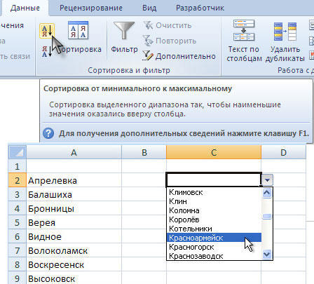
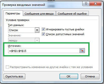
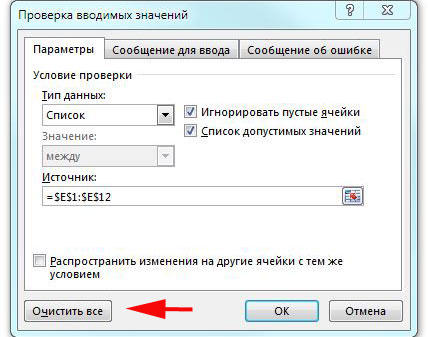
After you have formed a list of data, select the cell in which the drop-down list should be created. In the Excel Settings Ribbon, on the Data tab, find the Validate button. Clicking on it will open a dialog box. In it, you need to select the “Allow” item and set its value to “List”. So in this cell, the input method will be changed to a choice from the available options. But so far these options have not been determined. In order to add them to the created object, enter the data range in the "Source" field. In order not to type them manually, click on the input icon in the right part of the field, then the window will be minimized, and you will be able to select the desired cells with the usual mouse selection. As soon as you release the left mouse button, the window will open again. It remains to click OK, and a triangle, a drop-down list icon, will appear in the selected cell. By clicking on it, you will get a list of the options you entered earlier. After that, if the options are located on a separate sheet, you can hide it by right-clicking on its name at the bottom of the working window and selecting the item of the same name in the context menu.
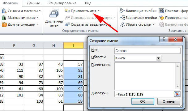
When you select this cell, several buttons will appear next to it. To make it easier for the user to enter, you can use this button to set the cell name. You can do the same above, next to the formula input box there is a corresponding item. So the list will be clearer, because the user will not have to guess by its values what exactly should be selected here. In addition, in the dialog box, you can enter a hint message that will be displayed when you hover over the cell. If the cell should not be left blank, uncheck "Ignore empty values". The "List of Valid Values" checkbox must be checked in any case.
Deleting a list
When the drop-down list is no longer needed, it can be removed from the document. To do this, select the cell on the Excel sheet containing it, and go to the Ribbon settings on the tab "Data" - "Data Validation". There, in the settings tab, click on the "Clear All" button. The object will be deleted, but the data range will remain unchanged, i.e. the values will not be deleted.
Conclusion
The algorithm for creating such objects is simple. Before you create a drop-down list in Excel, create a list of values, if necessary, format it as you like. Pay attention to 2 nuances. First: the length of the data range is limited, the threshold value is 32767 items, second: the length of the pop-up window will be determined by the length of the items from the list. By placing this object on the page, you will simplify the input of data from other users. Their use has a positive effect on the speed and accuracy of work, helps to simplify the formulas that work in the document, and solves the problem of unequal formatting of text data. But if you use Microsoft Share Point in an Excel workbook, it will be impossible to create a drop-down list, due to limitations in the work of the publishing program.