How to set up a drop-down list in Excel (Excel add make create)
How to create a drop-down list in Excel? Everyone has long known how well Excel works with tables and various kinds of formulas, but few people know that you can make drop-down lists here. And today we will talk about them.
And so there are several options for how to make drop-down lists for working in Microsoft Office Excel.
Option one is very simple. If you enter similar data in the same column from top to bottom, then you just need to stand on the cell below the data and press the key combination “Alt + down arrow”. A drop-down list will appear in front of you, from which you can select the data you need with one click.
The disadvantage of this method is that it is designed for a sequential method of data entry and if you click on any other cell in the column, the drop-down list will be empty.
Option two gives more opportunities, it is still considered standard. This can be done through a data check. First of all, we need to select the range of data that will go into our list and give it a name.

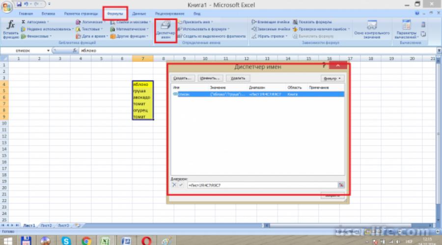
You can edit this range through the “Formulas” menu tab by selecting the “Name Manager” icon. In it you can create a new drop-down list, edit an existing one, or simply delete an unnecessary one.

The next step is to select the cell where our drop-down list will be placed and go to the “Data” menu tab, click on the “Data Check” icon. In the window that opens, we need to select the type of data that will be entered in our cell. In our case, we select “Lists” and below, through the equal sign, write the name of our range, and click OK. In order to apply the list to all cells, just select the entire column or the area you need before turning on data validation.

There are other more complex options for creating a dropdown list, such as: Inserting through the Developer menu tab, where you can insert dropdown lists as part of a form element or as part of an ActiveX control. Or write appropriate macros to create and operate drop-down lists.
Enter data in cells A1:A10, which will act as the source for the list. In our example, we entered numbers, they will appear in the drop-down list. Select the cell (For example, E5) that will contain the drop-down list. Select the Data menu -> Data Validation to open the Validate Input Values dialog box.
3. On the Options tab, select the List option from the drop-down menu. Make sure the correct boxes are checked.
4. Then, click on the button. The following dialog box will appear.
5. Select the items that will appear in the drop-down list on the sheet using the mouse, click on the button and return back to the “Validate input values” window, then click the “OK” button.
6. A drop-down list in Excel will be created.
If your list is short, you can enter items directly into Source in the Setup tab of the Validate Input dialog box. Separate each list item with the separators specified in the regional settings.
If the list needs to be on another sheet, you can use the "=List" option before specifying the data range.
How to create a drop-down list in Excel based on data from the list
Let's imagine that we have a list of fruits:
How to make a dropdown list in Excel
To create a dropdown list we will need to do the following steps:
Go to the “Data” tab => “Working with Data” section on the toolbar => select the “Data Validation” item.
In the “Source” field, enter the range of fruit names =$A$2:$A$6 or simply place the mouse cursor in the “Source” value entry field and then select the data range with the mouse:
If you want to create dropdown lists in multiple cells at a time, then select all the cells in which you want to create them and then follow the steps above. It is important to ensure that cell references are absolute (for example, $A$2) and not relative (for example, A2 or A$2 or $A2).
How to make a dropdown list in Excel using manual data entry
In the example above, we entered a list of data for a drop-down list by selecting a range of cells. In addition to this method, you can enter data to create a drop-down list manually (it is not necessary to store it in any cells).
For example, imagine that we want to display two words “Yes” and “No” in a drop-down menu.
For this we need:
Select the cell in which we want to create a drop-down list;
Go to the “Data” tab => “Working with Data” section on the toolbar =>
Validating Data in Excel
In the “Checking input values” pop-up window, on the “Parameters” tab, select “List” in the data type:
Validating input values in Excel
In the “Source” field enter the value “Yes; No".
Click “OK”
Not really
The system will then create a drop-down list in the selected cell. All elements listed in the “Source” field, separated by semicolons, will be reflected in different lines of the drop-down menu.
If you want to simultaneously create a drop-down list in several cells, select the required cells and follow the instructions above.
How to create a drop-down list in Excel using the OFFSET function
Along with the methods described above, you can also use the OFFSET formula to create drop-down lists.
For example, we have a list with a list of fruits:
In order to make a drop-down list using the OFFSET formula, you must do the following:
Select the cell in which we want to create a drop-down list;
Go to the “Data” tab => “Working with Data” section on the toolbar => select “Data Validation”:
Validating Data in Excel
In the “Checking input values” pop-up window, on the “Parameters” tab, select “List” in the data type:
Validating input values in Excel
In the “Source” field enter the formula: = OFFSET(A$2$,0,0,5)
Click “OK”
The system will create a drop-down list with a list of fruits.
How does this formula work?
In the example above, we used the formula =OFFSET(link,offset_by_rows,offset_by_columns,[height],[width]).
This function contains five arguments. The “link” argument (in the example $A$2) indicates which cell to start the offset from. In the arguments “offset_by_rows” and “offset_by_columns” (in the example the value “0” is specified) – how many rows/columns need to be shifted to display data.
The “[height]” argument specifies the value “5”, which represents the height of the range of cells. We do not specify the “[width]” argument, since in our example the range consists of one column.
Using this formula, the system returns to you as data for the dropdown list a range of cells starting with cell $A$2, consisting of 5 cells.
How to make a drop-down list in Excel with data substitution (using the OFFSET function)
If you use the OFFSET formula in the example above to create a list, you are creating a list of data that is captured in a specific range of cells. If you want to add any value as a list item, you will have to adjust the formula manually.
Below you will learn how to make a dynamic drop-down list that will automatically load new data for display.
To create a list you will need:
Select the cell in which we want to create a drop-down list;
Go to the “Data” tab => “Working with Data” section on the toolbar => select “Data Validation”;
In the “Checking input values” pop-up window, on the “Parameters” tab, select “List” in the data type;
In the “Source” field, enter the formula: = OFFSET(A$2$,0,0,COUNTIF($A$2:$A$100;”<>”))
Click “OK”
In this formula, in the “[height]” argument, we indicate as an argument denoting the height of the list with data – the COUNTIF formula, which calculates the number of non-empty cells in the given range A2:A100.
Note: for the formula to work correctly, it is important that there are no empty lines in the list of data to be displayed in the drop-down menu.
How to create a drop-down list in Excel with automatic data substitution
In order for new data to be automatically loaded into the drop-down list you created, you need to do the following:
We create a list of data to display in the drop-down list. In our case, this is a list of colors. Select the list with the left mouse button:
drop-down list with automatic substitution in Excel
On the toolbar, click “Format as table”:
Select a table design style from the drop-down menu
By clicking the “OK” button in the pop-up window, we confirm the selected range of cells:
Assign a name to the table in the upper right cell above column “A”:
The table with the data is ready, now we can create a drop-down list. To do this you need:
Select the cell in which we want to create a list;
Go to the “Data” tab => “Working with Data” section on the toolbar => select “Data Validation”:
In the “Checking input values” pop-up window, on the “Parameters” tab, select “List” in the data type:
In the source field we indicate = “the name of your table”. In our case, we called it “List”:
Source field automatic data substitution in Excel drop-down list
Ready! A drop-down list has been created, it displays all the data from the specified table:
In order to add a new value to the drop-down list, simply add information to the cell next after the table with the data:
The table will automatically expand its data range. The drop-down list will be replenished accordingly with a new value from the table:
Automatically inserting data into a drop-down list in Excel
How to copy a dropdown list in Excel
Excel has the ability to copy created drop-down lists. For example, in cell A1 we have a drop-down list that we want to copy to the range of cells A2:A6.
To copy a dropdown list with the current formatting:
left-click on the cell with the drop-down list that you want to copy;
select the cells in the range A2:A6 into which you want to insert the drop-down list;
Press the keyboard shortcut CTRL+V.
So, you will copy the drop-down list, maintaining the original list format (color, font, etc.). If you want to copy/paste a dropdown list without saving the format, then:
left-click on the cell with the drop-down list that you want to copy;
press the keyboard shortcut CTRL+C;
select the cell where you want to insert the drop-down list;
right-click => call the drop-down menu and click “Paste Special”;
dropdown list in excel
In the window that appears, in the “Insert” section, select “conditions on values”:
Click “OK”
After this, Excel will copy only the data from the drop-down list, without preserving the formatting of the original cell.
How to select all cells containing a drop-down list in Excel
Sometimes, it is difficult to understand how many cells in an Excel file contain drop-down lists. There is an easy way to display them. For this:
Click on the “Home” tab on the Toolbar;
Click “Find and Select” and select “Select Group of Cells”:
In the dialog box, select “Data Validation”. In this field you can select the items “All” and “The Same”. “All” will allow you to select all drop-down lists on the sheet. The “same” item will show drop-down lists with similar data content in the drop-down menu. In our case, we select “all”:
Dropdown list in Excel. How to find all lists
Click “OK”
By clicking “OK”, Excel will select all cells with a drop-down list on the sheet. This way you can bring all the lists to a common format at once, highlight boundaries, etc.
How to make dependent dropdown lists in Excel
Sometimes we need to create several drop-down lists, and in such a way that, by selecting values from the first list, Excel determines what data to display in the second drop-down list.
Let's assume that we have lists of cities in two countries, Russia and the USA:
To create a dependent dropdown list we need:
Create two named ranges for cells “A2:A5” with the name “Russia” and for cells “B2:B5” with the name “USA”. To do this, we need to select the entire data range for the drop-down lists:
dependent dropdown list in Excel
Go to the “Formulas” tab => click in the “Defined names” section on the “Create from selection” item:
Dependent Dropdown Lists in Excel
In the “Create names from a selected range” pop-up window, check the “in the line above” box. Having done this, Excel will create two named ranges “Russia” and “USA” with lists of cities:
dependent-drop-down-list-in-excel
Click “OK”
In cell “D2” create a drop-down list to select the countries “Russia” or “USA”. So, we will create the first drop-down list in which the user can select one of two countries.
Now, to create a dependent dropdown list:
Select cell E2 (or any other cell in which you want to make a dependent dropdown list);
Click on the “Data” tab => “Data Check”;
In the “Validate input values” pop-up window, on the “Parameters” tab, in the data type, select “List”:
Validating input values in Excel
Click “OK”
Now, if you select the country “Russia” in the first drop-down list, then only those cities that belong to this country will appear in the second drop-down list. This is also the case when you select “USA” from the first drop-down list.