Print the table header on each page. How to print headers (names) of rows and columns on each page in Excel

Most often, Microsoft Excel is used to create tables, since the default sheet is divided into cells, the size of which can be easily changed to a suitable size, and rows can be automatically numbered. In this case, at the top of all data there will be a so-called header, or column headings. When printed, it will definitely appear on the first page, but what about the rest?

We will deal with this in this article. I’ll tell you two ways to make sure that when printed, the title and headings in the table are repeated on every page in Excel, and how to increase the font, size and color for them.

Using through lines

The first way is to use through lines. In this case, you need to add additional rows above the table, one or more, and enter the required text in them.

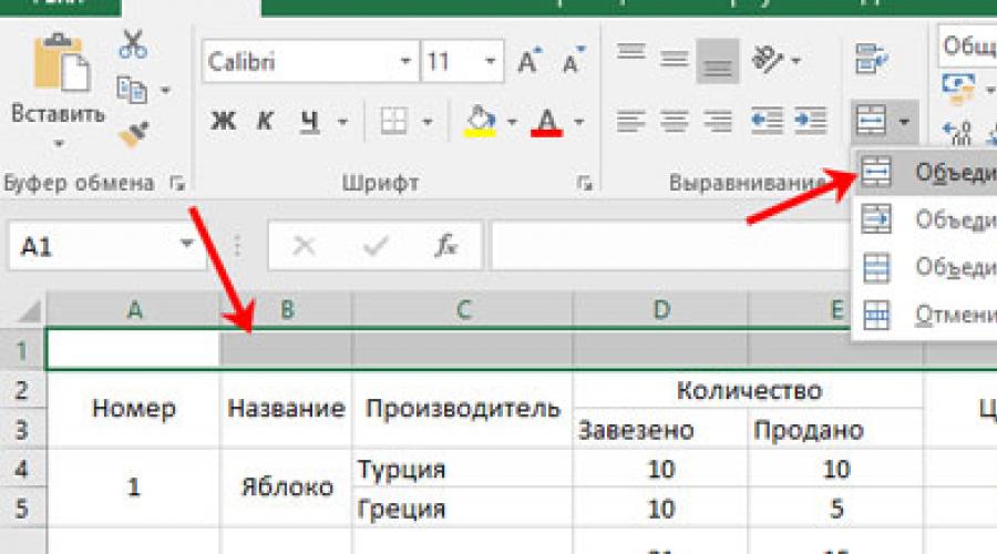
Select any cell from the first row and, being on the "Home" tab, click "Insert". Then select from the list "rows per sheet".

Next you need to make one from several blocks. To do this, select those that are located exactly above the table, click on the corresponding button and select from the list either simply “Merge”, or with placement in the center.

You can now print a title for the table.

Then move on to formatting it. For this you can use the buttons located in the “Font” group. I made the general title larger, changed the font and added a background. I also made the column names on a gray background and applied italics to them.

After that, open the tab "Page layout" and press the button "Print Headers".

A window like this will open. Put italics in the box "through lines".

Next, click on the first row (where the number 1 is) and drag down the required amount. In the example, the repeating heading corresponds to the first, second and third row. In this case, a small field will show what you are highlighting.

We return to the familiar window and click “OK” in it.

To see what we did, click “File” at the top and then select “Print” on the left.

The preview window will show you what the printed page will look like. As you can see, there are headings on the first sheet.

Using headers and footers

The second way is to add headers and footers. Since our header is already repeated, we did this in the previous step, let's now duplicate the general name of the table on all sheets.

Open “View” at the top and go to mode "Page layout".

The header field we need will appear at the top of the page, click on it.

If it doesn't appear, place italics on the line between the pages and click on it to show the empty space.

The footer is divided into three parts. Type the appropriate text in one of them. In the example, I will print the table name in the center. Then select it and, using the buttons on the "Home" tab, you can increase the font, change the color, add boldness or italics.

When finished, switch from markup mode to normal.

Let's see what we got. Using the method described above, go to “File” - “Print”. The first page contains both the title and the name of the table.

In these ways, you can add a table title to each page in Excel when printing. Use the option that is most suitable for solving your problem.

Let's learn attach the table header as a heading for printing(with fixed rows or columns) on each page in Excel.

How often have you scrolled down or to the right and lost sight of the title?
If you fix the table header using freezing areas, then when scrolling the Excel sheet, the header will indeed remain motionless and the problem is solved, but when printed it will still not be repeated on each page, which can lead to incorrect interpretation of the data (you can easily confuse the data due to incorrect designation).

And then, in order to understand which row or column of data is responsible for what, you will have to return to the beginning of the sheet, which is extremely inconvenient. Therefore, if the printed document takes up more than one page, then repeating the headings will greatly simplify the reading of the document.

How to attach a heading to every printed page in Excel?

Excel has standard tools that allow you to make a repeating table header when printing a document.
But first, let’s decide what type of header we will need to work with; in general, there are two types:

• Horizontal. The header is located at the top and the body of the table is at the bottom;
• Vertical. The header is on the left and the body of the table is on the right.

There is only one difference in working with different types of headings - for horizontal ones we will make only the rows motionless, and for vertical ones - columns.
Let's move on to practice and use examples to look at how you can print a header in Excel so that it appears on every sheet.

How to fix a horizontal header?

Let's consider a large table (let's take one so that it probably won't fit on one page) with a horizontal header (rows 1-2 with the name of the table and the designation of the data contained in it), which we subsequently plan to print:

To see how the sheet will look when printed, you can use the preview (on the tab bar File -> Seal, or using Ctrl+F2).

As you can see, on the first sheet the header in the table is located at the top, but on the second it is not there at all, which makes it unclear what kind of data is in which column (for example, by looking only at the second page it is impossible to determine what exactly the data shows):

Now let's move on to setting the sheet printing parameters.
On the tab bar, select a tab Page layout and in the section Page settings press Print headings:

In the pop-up window (you can also customize the output here), we are interested in the block where we can set end-to-end rows and columns.
Name end-to-end precisely implies that these elements will pass through all printed sheets:

Accordingly, if the table header is presented in horizontal form, then in order to make the header motionless when printing the page, we need to set the dockable area as end-to-end rows.

Select the lines to pin (in this case, these are lines 1 and 2, i.e. enter $1:$2 ), and then click the view button to display the changes made:

As you can see, headings also appeared on the second sheet of the table, just like on the first.

Everything is ready, you can send the document for printing.

How to attach a vertical header?

Let's consider another case when the table header is located not horizontally, but vertically (column A with a list of employees):

First, let's check what our table looks like when printed.
Using the preview, we make sure that the heading on the second page is missing:

Let's repeat all the steps from the previous example (when we fixed the rows), but at the last step, instead of end-to-end rows, we will set end-to-end columns.
In this case, we need to fix the first column, so in the field Through columns enter $A:$A. As a result we get:

As we can see in this case, a floating header appeared on each sheet; now the document is also completely ready for printing.

Thank you for your attention!
If you have thoughts or questions on the topic of the article, share them in the comments.

Let's consider To How to fix a table title in Excel, how to setup Print rows and columns on each Excel page, freeze the top rows and columns. How to freeze a table header in Excel so that when scrolling a large table, the table header is always visible, etc., read the article “How to freeze a row and column in Excel.”
How to print a table header on every Excel page.
To print a table header on each page, go to the “Page Layout” tab in the “Sheet Options” section and select the “Page Options” function. This button is located at the bottom right of the Sheet Options section - it's a small button with an arrow.
This button is circled in red in the image. In the window that appears, go to the “Sheet” tab.
In the “Print on each page” section, in the “through lines” line, set string range(table headers). Here in the picture the range of one line is indicated.
In order not to manually write the range, you can make it simpler. Place the cursor in the line “through lines” (click the mouse) and go to the table. Select all the rows of the table header, the address will be written automatically.
The header range in the table will be outlined with a pulsating dotted line (see image). Here you can immediately see how it turned out. To do this, click the “View” button. If everything suits you, click the “OK” button.
Print columns on each Excel page.
In the same way as rows, you can set the range of columns that should be printed on each page.
You can put the address of a column (or row) simply. Place the cursor in the line “through columns”. Then, click with the mouse on the column address (letters, A, B, etc.), this column will be highlighted, its address will appear in the “through columns” line. You can select several columns at once. Using this principle, we select rows by clicking on the row address line, “1”, “2”, etc.).
If in the Print section of the window If we check the “grid” function, the Excel sheet grid will be printed with a gray dotted line (where the cell borders are not drawn).

If you have created a large table in Microsoft Word that occupies more than one page, for ease of working with it, you may need to display a header on each page of the document. To do this, you will need to set up automatic transfer of the title (the same header) to subsequent pages.

So, in our document there is a large table that already takes up or will only take up more than one page. Our task is to configure this table in such a way that its header automatically appears in the top row of the table when you go to it. You can read about how to create a table in our article.

Note: To move a table header consisting of two or more rows, you must also select the first row.

1. Place the cursor in the first row of the header (first cell) and select this row or rows that make up the header.

2. Go to the tab "Layout", which is in the main section "Working with tables".

3. In the tools section "Data" select an option.

Ready! With the addition of rows in the table that will carry it to the next page, the header will be automatically added first, followed by new rows.

Automatic wrapping of not the first row of the table header

In some cases, the table header may consist of several rows, but automatic wrapping only needs to be done for one of them. This, for example, could be a line with column numbers located below the line or lines with the main data.

In this case, we first need to split the table, making the row we need a header, which will be transferred to all subsequent pages of the document. Only after this will it be possible to activate the parameter for this line (already the header) "Repeat Header Rows".

1. Place the cursor in the last row of the table located on the first page of the document.

2. In the tab "Layout" ("Working with tables") and in the group "An association" select option "Split table".

3. Copy that line from the “big” main header of the table, which will act as a header on all subsequent pages (in our example, this is the line with the names of the columns).

Advice: To select a line, use the mouse, moving it from the beginning to the end of the line; to copy, use the keys "CTRL+C".

4. Paste the copied row into the first row of the table on the next page.

Advice: Use the keys to insert "CTRL+V".

5. Select the new header with the mouse.

6. In the tab "Layout" click on the button "Repeat Header Rows" located in the group "Data".

Ready! Now the main table header, consisting of several lines, will be displayed only on the first page, and the line you added will be automatically transferred to all subsequent pages of the document, starting from the second.

Removing the header on each page

If you need to remove the automatic table header on all pages of the document except the first, do the following:

1. Select all the rows in the table header on the first page of the document and go to the tab "Layout".

2. Click the button "Repeat Header Rows"(group "Data").

3. After this, the header will be displayed only on the first page of the document.

We can finish here, from this article you learned how to make a table header on each page of a Word document.

Microsoft programs are popular because they are convenient both for working with office documents and for personal purposes. Excel is a program that has a large number of different functions that allows you to work with large and massive tables, even on weak computers. In order to understand all the functionality, you need to spend a lot of time, so next we will talk about how it is possible to attach a header in Excel.

How to attach a header in Excel

This can be done either with the help of a special tool that will allow you to print it on each page, or with the help of another that allows you to secure the top line, and when scrolling, the line will be displayed constantly at the top. You can attach the leftmost column in the same way. How can this be done?

In Excel 2003/2007/2010

To attach a header in Excel 2003, 2007 or 2010, you need to follow a few simple steps:

In Excel 2013/2016

In Excel 2016, everything is done in a fairly similar way. Here are step-by-step instructions for pinning in the new Excel:

With this pinning, a row or column will always be visible, which is quite convenient when working with large tables, since scrolling them down in standard mode hides the header.

How do I attach a header to each page for printing?

In the case when you need to print such a line on each page, you need to do the following:

After these operations, when printing, the header will be displayed on each of the printed sheets; you can print the entire table.

Based on this, making pins in Excel is actually quite simple, for which you just need to remember the sequence and what operations need to be performed, and then working in Microsoft Excel will bring you nothing but pleasure.

Video: How to attach a header in Excel?